Wehrl entropy production theory for non-equilibrium quantum systems

In Chapter 6, we apply our formalism to the dynamics of the KBM model under quantum quenching. We study the Gaussianity of the state during the dynamics and the Wehrl entropy rate components.

The postulates of quantum mechanics

Modern quantum mechanics for isolated systems can be summarized by four postulates, which are the subject of the next section. When dealing with a physical system, we are often interested in quantities that can be measured in a laboratory, these are called observables and are associated with special set of operators.

Open quantum systems

Exemple 1: Dynamics of a single qubit

In this case the population remains constant again, but over time the coherence of the system is washed away. This simple example sheds light on the role of the environment for quantum system, it is responsible for decoherence which occurs exponentially in timee−4κt, for this example.

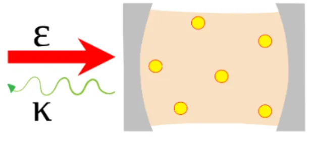
Exemple 2: Driven-dissipative quantum harmonic oscillator at

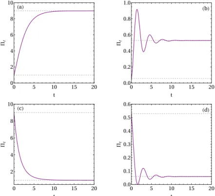
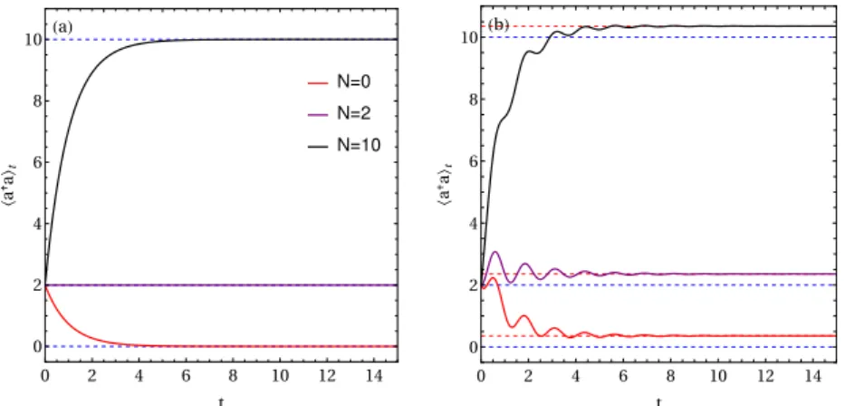
In this case, it is more informative and possible to study the evolution of some observables rather than the dynamics of the state itself. In Fig.1.2(a) we see the dynamics of the number of quantum ha†ai of a quantum harmonic oscillator, E = 0, which is subject to dissipationκ.

Coherent states

A coherent state can be expressed in number states |ni, which are the eigenstates of the number operators†a|ni=n|ni, which,. This result shows that the diagonal elements of the coherent state basis fully determine all matrix elements of O, since:.

Quantum mechanics in phase space: The Husimi Q-function

Finally, the average of the anti-normally ordered products of the creation and annihilation operators is given by . It is straightforward to generalize the above results for any number of applications of the operators, for example ariρ→(µi+∂µ¯i)rQ(µi,µ¯i).

Heterodyne measurements

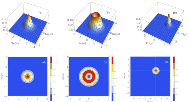
Examples of the Husimi Q-function

In addition to the entropy exchanged with the reservoir, entropy can also be spontaneously generated in the process. From which the efficiency of the machine will be less than the Carnot efficiency due to the entropy production.

Entropy production and non-equilibrium steady states

Entropy production for quantum systems

Example of a QPT: the Lipkin-Meshkov-Glick model

Spin coherent states share the same peculiarity: they make the average of spins equal to classical spins. S= (hJxi,hJyi,hJzi) =j(sinθcosφ,sinθsinφ,cosθ), (3.8) wherehJii,i=x, y, z is the average of the macrospinJitaken with respect to the state (3.7). The term θδ(σ0i, σi) is the local spin dependence, proportional to the inertial termθandσi0 represents the spin of the majority neighborhood.

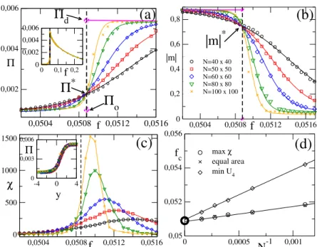
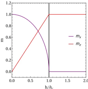
Panel (a) and (b) respectively show the NESS entropy production and the order parameter|m|near the critical parameter f0, the inset shows the behavior of the NESS entropy production over a wider range, we see that the entropy production is finite and has a discontinuity. Panel (c) is the plot of the variance χ = N(hm2i − |m|2) near the critical point. We note that as the volume N increases, the variance shows a finite peak approaching f0. In (d) the graph of the maximum of χ, the minimum of U4 and the probability distribution of the equal area order versus N−1.

Surprisingly, we will encounter a similar behavior, as shown in the insets of Fig.3.2 for one of the contributions to the entropy production in the quantum context at the end of Chapter 5.

Driven-dissipative phase transitions

Application: driven-dissipative quantum harmonic oscillator

The eha†aiSS value can easily be found by writing the time evolution for the moments (we repeat these equations for the sake of clarity). In case we have a driven-dissipative cavity ∆ = 0 we find that ΠSS = 2E2/κ, which is similar to the entropy product of the RL circuit discussed in 2.2, ΠRL = E2/RT. It is important to note that, although the results have the same structure, the physical processes behind them are quite different, in the RL circuit both energy and dissipation occur incoherently, while in the driven cavity the energy input is coherent.

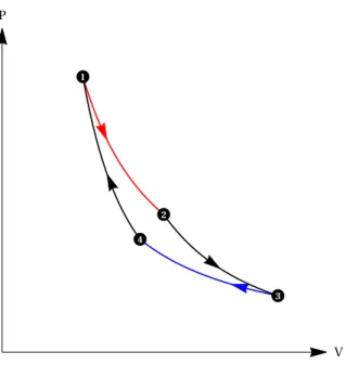
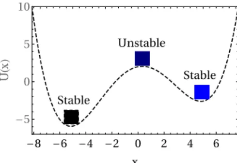
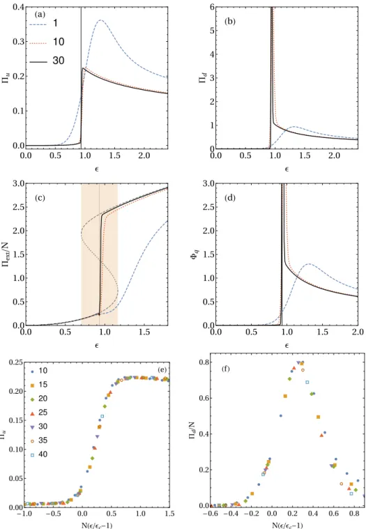
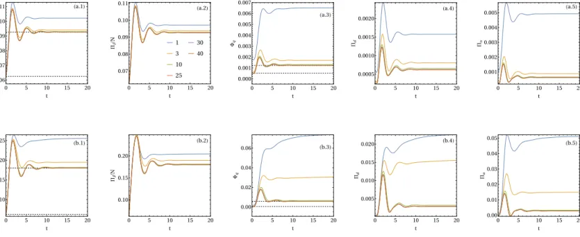
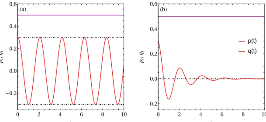
To illustrate this, we consider the damping scenario for its simplicity: we choose an initial E0 and let the system relax to the appropriate NESS, then at time t = 0 the amplitude suddenly changes to Ef, the time evolution of the system is given by solving the Lindblad equation with this new parameters. During transient dynamics, the entropy production becomes greater (lower) than the NESS entropy production, for which the system will relax. In the case Ef

Thermodynamic limit in critical systems

Properties of the unitary contribution to entropy production

To understand the physics of the unitary contribution to the entropy production rate given by Eqn.(4.12) we will consider the case of a system described by a normal Hamiltonian ordered in a single order,. These are the key unitary dynamics terms in the thermodynamic limit in the quantum Fokker-Planck equation. Here, a characteristic feature of the Husimi function Q stands out, which are the terms of the second derivatives, interpreted as diffusive terms.

Between them there is always a local maximum, which is the unstable equilibrium point, in the sense that any disturbance causes the system to go to one of the minima and it can be interpreted as a barrier between minima. The effect of the non-linear medium is to promote an effective interaction between the photons with strength U. The cavity is driven coherently by a laser with an amplitude E, which will behave like a classical field. Before studying the Wehrl entropy production rate, we will provide further details of the model.

The last term is due to the non-linearity of the medium and describes the effective interaction between the photons in the cavity.

Dynamical equations for the moments

Mean Field approximation

It is only valid if the number of photonsha†ai=|µ|2 in the cavity is "very high", so that the interaction strength U becomes very weak. It is interesting to note that (5.8) and (5.13) have the same structure and, from a mathematical point of view, the same properties; in the next section we consider the stability problem of this equation. To know what the conditions are for stable solutions to the equation. 5.8) in the long-term limit → ∞where the system reaches NESS, we will perform the linearization procedure (see app.

To simplify the notation along this section, we set|α|2=n so that NESS can be summarized by the equation,.

Stability analysis of the steady state

In this case, due to the minus sign of J, a stable solution requires both eigenvalues ​​to be positive. The first condition gives us thatTr{J}= 2κ >0, so the dissipation rate must be positive, which is consistent with the Lindblad formalism. From the first term we see that ∆/u <0, butu is accepted as positive due to its physical interpretation of an interaction strength between the photons, thus ∆<0.

This condition tells us that to have a bistable behavior we must have the cavity frequency to be less than the pump frequencyωc < ωp.

Exact solution for the moments

On the coherent quantum absorber method

The Born-Markov approximation is assumed to be valid for this system coupled to the waveguide so that the cascade master equation for the reduced system density matrix is ​​ρ,. Manipulate the terms of (5.28) and define c=P. c†jci−c†icj) (5.30) is the cascade Hamiltonian with nonlocal coherent dynamics of the coupling mediated by the environment. To apply the method for the KBM model, we consider a network consisting of two subsystems A and B.

This ensures that no photons leak out of the waveguide and will allow the system to relax to a pure stateρ0 =|ψ0i hψ0|[112]. For the KBM we have,. to make up the systemHB we make use of the educated guess used in Ref. Since|ψ0i is a tensor product and the symmetric mode is in the vacuum state, the non-zero normal. ordered operator is that of the anti-symmetric mode.

The main advantage of the CQA method is that it reduces the problem to a simple recursion formula Eq. 5.44), instead of solving a Fokker-Planck equation for the P representation, which is much more complicated from a mathematical point of view.

The Wehrl entropy production rate for the Kerr bistability model

Such a behavior matches experimental observation of the irreversible entropy production in mesoscopic systems, reported in Ref. Moreover, a finite size scaling analysis of Πu and Πd ensures the universality of the results for the thermodynamic limit. 4 was able to capture some interesting features of entropy production at the NESS of the KBM model, as reported in Ref.

With this in mind, we first study the Gaussianity of the state during the dynamics and show that unfortunately this is not the case with our system. This means the Hamiltonian isat most quadraticinaianda†i which is not the case of the KBM model Eqn.(5.2), since it has a terma†a†aa interaction. If the state of the KBM model were Gaussian during the dynamics, we could easily obtain all the entropic quantities using eqn (6.6) in Eqns.

Stands for the critical pump amplitude and + is the upper limit of the bistable region as found by MFA in Eq.(5.13).

Entropic dynamics in a quench scenario: results and discussion

The unitary contribution behaved qualitatively similar to that of the entropy production in classical non-equilibrium transitions explained in Sec. Another line of research is to better understand the behavior of the unitary contribution to the entropy production rate. In the next section we show the details for the KBM of the main text.

We note that it is always centralized and zero in the bounds, as required to compute the integrals of the entropy production rate numerically. Using quantum phase-space methods, we have developed a framework that allows the complete characterization of entropy production in driven-dissipative transitions. In this system, the part of the entropy production resulting from quantum fluctuations at the critical point was found to diverge [45].

This part of the entropy production is continuous, but has a kink (discontinuous first derivative) at the critical point λc=. The entropy production rate in Eq. 6) of the main text has a term proportional to the unit dynamics, . These are the leading-order contributions of the unitary dynamics to the Fokker-Planck equation.