However, in articles in which multiple observations are clustered at locations that are close to each other, such as households in cities by Dell (2010), the standard errors originally reported are major underestimates. Most importantly, and this cannot be stressed enough, this article is not concerned with "confirming" or "refuting" the findings of any particular study in any way. Usually, the regression examined is the main regression of the article, including the additional robustness variables added by the authors.
3 Fitting Spatial Noise
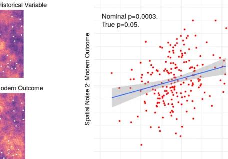
Now suppose we take two noise processes and evaluate them in each city, then backtrack to each other. In fact, the empirical significance level is 5 percent (out of 1000 random noise regressions, its p-value was at the 5th percentile): the estimated t-statistic is twice its correct value. The inflated statistic is the result of our failure to adjust standard errors for the fact that only about a quarter of the observations in this case contribute anything useful to the accuracy of the coefficient estimate.
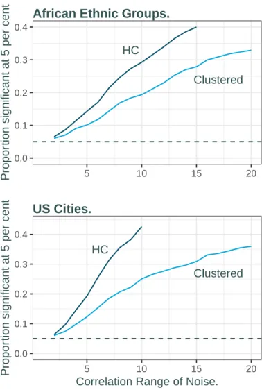
These inflation values are shown systematically in Figure 5, where the points are now based on the African ethnic groups used by Michalopoulos and Papaioannou (2013) and US commuting zones from Chetty et al. 2014), where the original coordinate axes have been changed to make each 100×100 square. The statistics are noticeably inflated even for moderate areas of spatial correlation, in a manner that differs across datasets. At an interval of 10, almost one-third of the African regressions are significant using HC standard errors, and 40 percent of the American ones.
As mentioned earlier, by clustering we use a procedure to protect against spatial correlation, which should not be used in the presence of spatial correlation. When standard errors are clustered, the proportion of significant regressions is roughly halved, but inflation is still substantial.
4 Spatial Kernel Estimation
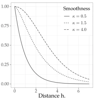
For the studies analyzed here, correlation between residuals tends to decline exponentially with distance, corresponding to κ= 0.5. The parameterθ is a range parameter that controls how quickly correlation decays with distance, and κ is a smoothness parameter. The flexibility of the Matérn function is illustrated in Figure 6 where range θ is set to 1 and smoothness κ takes values from 0.5 to 4.
Because the Matérn function is monotonic, one can choose a distance beyond which the correlation is negligible and can be set to zero. This gives us a compact support for K and, assuming that this intercept distance is of the order oL1/3 where is the length of the study space, allows the kernel to satisfy the sufficient conditions of Conley (1999) that the estimated standard errors ( 1) be consistent. . Similarly for panels, if is the correlation matrix between the residuals across different time periods and Kis the spatial correlation each period, then the longitudinal kernel is the Kronecker product of the two.
A relevant concern for any such exercise is that the estimated standard errors will be substantially biased if the spatial correlation of the residuals differs from the assumed functional form, if the relevant economic locations of the observations differ from the geographic ones, or if the strength of the correlation varies with direction.
5 Persistence Studies: Adjusted Standard Errors
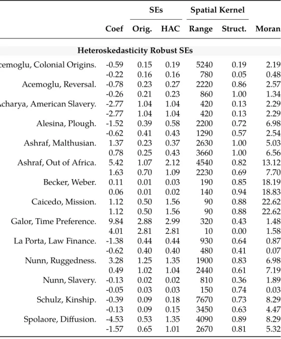
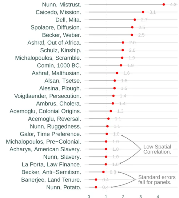
Appendix A presents Monte Carlo simulations which show that even substantial deviations from these assumptions lead to standard error estimates that are biased downward by less than five percent. time of the spatial range and structure parameters for the regression residuals. A property of the Matérn function is that when two places are separated by a distance=√. 8κ θ, the correlation between them is 0.14: this distance is usually called the effective range. In the second row, since robustness checks have often removed significant spatial structure, the difference between the original and adjusted standard errors is often lower, reflecting smaller kernel parameters and reduced Moran statistics.
Each row reports the original and adjusted standard errors along with estimated kernel parameters—effective range2θand spatial structureρ—and Moran statistics. The reason is that fixed effects have already absorbed a large part of the spatiotemporal structure of the residuals, so that clustering is an aggressive solution to a problem that. The spatial correlation parametersθandρfor panels, as well as Moran statistics, were calculated as the average of the values estimated for each period, and temporal autocorrelation was similarly an average of the autocorrelation between residuals in each period.
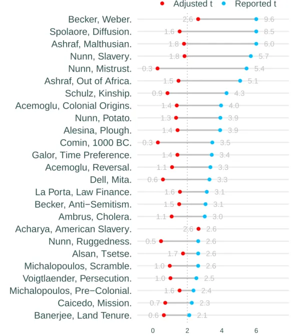
Again, large changes in the assigned kernel parameter values did not materially affect standard errors. It is increasingly recognized that because t-statistics confound the size of effects with how precisely those effects are estimated, they are not a useful measure of the importance of a variable.
6 Conclusions
Nevertheless, given the importance many of these studies seem to place on significance levels, it might be useful to see how robust they are. The risk of chasing spatial trends can be reduced by following the robustness checks applied above. Areas with particularly high values of the explanatory or dependent variables should be emphasized and the effect of removing them should be made explicit.
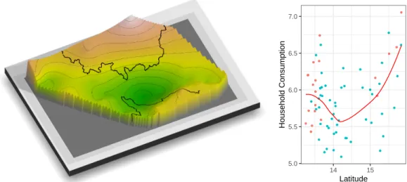
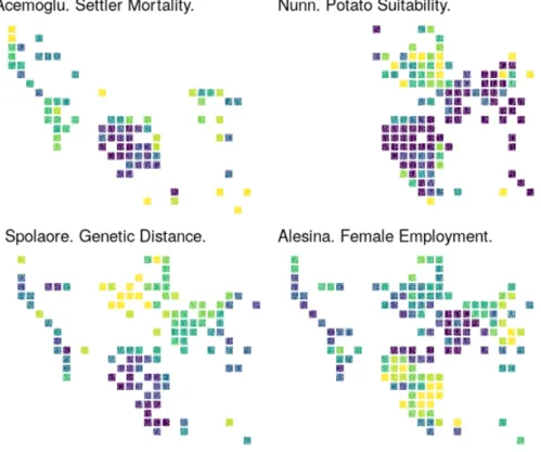
Given their unusual fragility, global studies based on country-level data should be undertaken with great caution. It is always advisable to be skeptical of any claimed regression results where a scatterplot of key variables is not provided. But with spatial data it's just as important to see simple color maps of the dependent and explanatory variables along with the residuals to quickly understand whether a regression fits something deeper than spatial trends.
Loss in the Time of Cholera: Long-Term Impact of a Disease Epidemic on the Urban Landscape." American Economic Review110:475-525. History, Institutions, and Economic Performance: The Legacy of Colonial Land Tenure Systems in India." American Economic Review. Religion, Division of Labor and Conflict: Anti-Semitism in German Regions over 600 Years.” American Economic Review.
Spatial correlation robust inference to errors in location or distance.” Journal of Econometrics 140:76–96. Identification and estimation of econometric models with group interactions, contextual factors and fixed effects.” Journal of Econometrics140:333–374. The Potato's Contribution to Population and Urbanization: Evidence from a Historical Experiment." Quarterly Journal of Economics126:593–650.
The Mission: Human Capital Transfer, Economic Persistence and Culture in South America.” Quarterly Journal of Economics134:507–556.
Appendix A Robustness of Standard Error Esti- mates
Errors in the Assumed Kernel
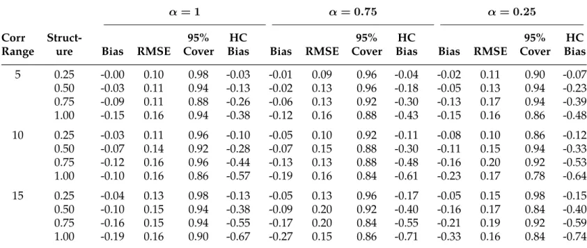
So the goal is to see how far the standard error for the yonx regression estimated with the Matérn kernel deviates from the correct value. Starting with the Cauchy case in Table A1 , Matérn's standard error is biased downward, reflecting the much larger spatial structure of the Cauchy residuals. Nevertheless, at shorter ranges and/or lower spatial structure, its performance is not very wrong, with a downward bias below 10 percent, even with a slow decay of α = 0.5.
The Matérn kernel again works well as long as the degree of spatial structure, this time controlled by λ, is not too high. Bias, Root MSE and 95% CI coverage probability level when a Matérn kernel is applied to residuals with Cauchy correlation. Bias, Root MSE and 95% CI coverage probability when a Matérn kernel is applied to data with spatial autoregressive structure with coefficientλ.
The fairly robust behavior of the Matérn kernel when applied to residuals with extremely slow and empirically unrealistic decay in correlation indicates that it should be reliable in cases where the data have a more realistic spatial structure. For example, if the true kernel follows a power exponential distribution (stable law) where C(si, sj;θ, γ) = exp(h/θ)−γ, the bias of the Matérn kernel is smaller and the results are not reported.
Errors in the Assumed Location of Observations
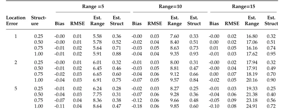
We can see that the overall bias is small when the distance is 1 or 2, but becomes significant at 5 when the spatial structure of the residuals is above 0.5. The table gives, in addition to the bias, the average range and structure calculated from the observed points: the structure is estimated quite accurately, but the range tends to be overestimated: this acts to moderate the downward bias of the estimates.
Anisotropy
Estimated bias, RMSE, structure, and range when observations differ from their true location by Gaussian noise with a mean distance of 1, 2, and 5.
Appendix B Alternative Standard Error Correc- tions
Bias, Root MSE and 95% CI coverage probabilities, when the residuals are geometrically anisotropic with a ratio of major to minor axis of 1.5 or 2; and the major axis runs at 0 or 45 degrees to horizontal.
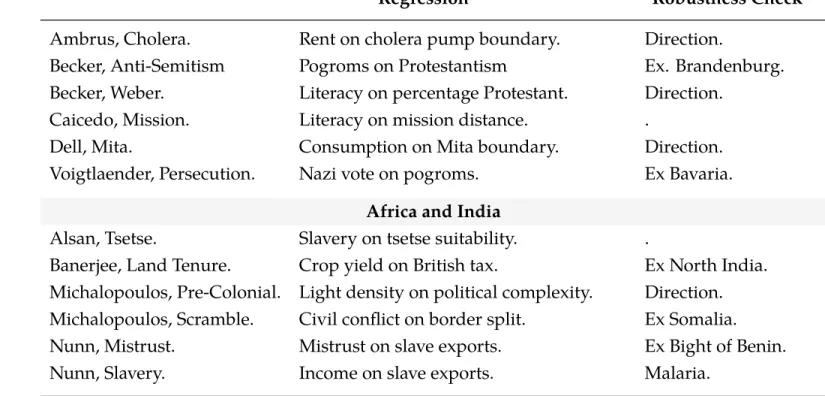
Appendix C Studies Examined
Study 2
- Global
- Africa and India
- Europe and the Americas
We replicate column 1 of table 3 in Acemoglu, Johnson, and Robinson (2002), regressing GDP per capita in 1995 on urbanization estimated at 1500. This replicates column 2 of Table 6, a regression of Judicial System Efficiency on a civil law model. controlling for GDP per capita. We analyze the final column of Table 1, where income is regressed on the interaction between terrain roughness and a dummy for African countries with added geographic controls.
This replicates the regression of individualism on kinship intensity from the top row of Table 2. We examine the baseline regression of pr. capital income on a measure of a country's genetic distance from the United States in the first column of Table 1. We take the regression in Column 1 of Table 3 of the yield of 15 major crops on the share of land controlled by landlords, along with geographic control and how long the area was under British rule.
We examine the baseline regression of night brightness on pre-colonial political centralization in Column 1 of Table 2. We analyze column 2 of Table 2 where literacy across Prussian provinces in 1871 is regressed on the percentage of the population that is Protestant.