Principles of a ground penetrating radar survey
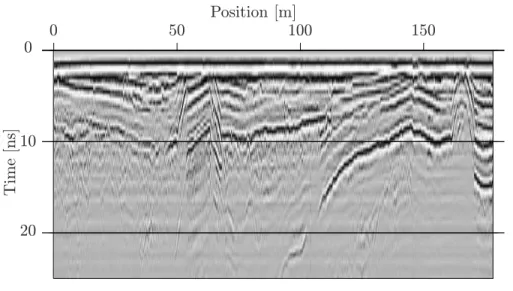
This research was carried out on a 200 m long highway section to determine the thickness of asphalt layers. These wave speeds can be determined by correlating the arrival times of the reflected waves in the data with the thickness of the asphalt cores.

Reason for the research
The most important parameter needed to get a good picture of the subsurface is the (frequency-dependent) wave speed. The polarization of the electromagnetic field manifests itself in the dipole nature of the source and receiver antennas.
Scientific strategy
Similar radiation characteristics of the source antenna can be used to describe the performance of the receiver antenna. The influence of the limited acquisition plan and the radiation characteristics of the source and receiver antennas on the spatial sampling criterion was investigated.
Outline of the thesis
Indeed, the multi-component imaging algorithm leads to a circularly symmetric resolution function of the point scatterer. In Chapter 7, the results of the experiments show the imaging results using the multi-component imaging algorithm.
The boundary conditions
For a medium that is also homogeneous, the scalar conductivity σ, the scalar permittivity ε and the scalar permeability µ are constants and so are the constitutive relations.
The Laplace transformation
Now we define the one-sided Laplace transform of some causal space-time quantity f(x, t) as. 2.12) A function in the time domain can be reconstructed from its Laplace transform by explicitly evaluating the Bromwich integral, which acts as the inverse Laplace transform. Simple rules of the one-sided Laplace transform apply, such as replacing ∂t by sand replacing a convolution of two time-domain quantities by the product of two complex s-domain quantities.
The temporal Fourier transformation
The spatial Fourier transformation
Transition to polar coordinates
Reciprocity theorem of Lorentz
The ω-domain wavefield reciprocity theorem
Equation (2.32) is the local form of Lorentz's reciprocity theorem. 2.32) over the domain ID and using Gauss's theorem on the resulting left-hand side leads to. First of all, it is noted that the first and second terms on the right-hand side of Eq. 2.33), disappear if the media in both states are chosen such that ˆηA= ˆηB and ˆζA= ˆζB.
The limiting case of an unbounded domain
These eigenfunctions are used to compose the wavefield solution from the set of upgoing and downgoing waves. Note that the vertical wavenumbersλn3(kα, ω) are the eigenvalues of the system matrix A, while the polarization vectors Fn(kα, ω) are the eigenvectors of the system matrix A.

Bi-orthogonal relations for eigenfunctions
The amplitude of ascending or descending waves W have a x3 dependence according to Eq. which shows that there is no interaction of waves propagating in the same direction and thus Eq. 3.40) where we have written the matrix B as a function of B↓↑ to implement real-valued normalization constants for N. There are different ways to choose the normalization constant contained in the matrix N. In this way the transmission and reflection coefficients, of which will be derived are equal to the results in the literature.
Scattering theory
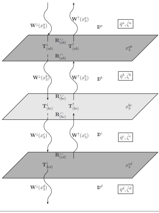
Next, we define the local reflection and transmission coefficients of the interface in terms of the local scattering operator of the interface S(xa↓3 ;xb3↑), expressed as. Evaluating the reflection and transmission coefficients using Eqs results in upward and downward reflection coefficients given by

The presence of sources on an interface
Sources at an artificial interface
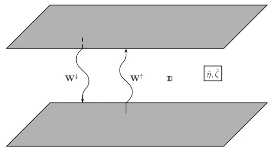
This will be important when performing a limiting procedure to obtain expressions for the sources present at the interface between two different media, which will be discussed later. When a source is present at the interface and there are no other interfaces, it is clear that only ascending waves are present forxb3 < xb3↓ (W↓(xb3) = 0), and that only descending waves are present forxc3 > xc3↑( W↑(xc3) = 0).
Sources at an interface between two different media . 45
In the first case the medium. parameters of IDb and IDc are equal to the medium parameters of IDa, resulting in . 3.67). No approximation can be made for the wave propagation regime and the full half-space matrix must be evaluated.
Electromagnetic field expressions in the horizontal wavenumber
Electromagnetic field in two homogeneous half-spaces 52
Note that only upgoing waves are present in the upper medium, denoted by the . propagation constant Γ0 which is present in the exponent for the emerging waves. Only downgoing waves are present in the lower medium, which is indicated by the propagation constant Γ1, which is present in the exponent for the downgoing waves.
Analytical derivation of closed-form expressions in the space-
Electromagnetic field in homogeneous space
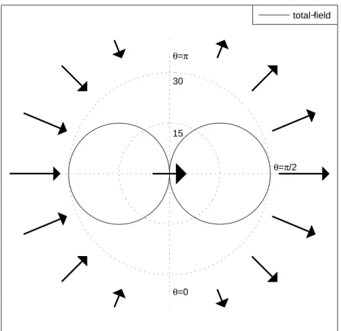
Note that all three electric field components will be present when they are not in the E or H plane. The only electric field component in the H plane is in the i1 direction and is omnidirectional.

Electromagnetic field in two homogeneous half-spaces
A summary of closed form expressions for the diffusive field for various sources on the surface of a homogeneous half space are summarized by Nabighian [1991]. For ground-penetrating radars, we are interested in closed-form expressions in the spatial frequency domain for Eqs.
Asymptotics for electric field generated by a horizontal electric
King and Smith [1981] investigated the validity of expressions for field values near the interface given by Ba˜nos for the joint diffusive and propagating regime and concluded that within a certain range the asymptotic solutions were valid. This results in the terms being complex conjugates of each other in the space-frequency domain.
Numerical evaluation of the integral expressions
This indicates that the intermediate field expressions given by Ba˜nos can be used for the lossless case. By analyzing the expressions for the electric field, two branch points can be identified in the complex wavenumber domain.
Validation of the asymptotic expressions for the electric field 68
A comparison between the far-field expressions and the combination between far- and intermediate-field expressions with the total-field evaluation, shows that interference of the body wave and head wave in the ground leads to a lobed structure. A comparison between the far-field expressions and the combination of far- and intermediate-field expressions with the total-field evaluation shows that interference of the body wave and head wave in the ground results in a lobed structure.

Forward scattering problem
In the cases xR ∈ ID, the integrals should be interpreted as their principal Cauchy values. To solve this system of integral equations, first ˆEkand ˆHjcan, in principle, be determined by taking x∈IDsin Eqs. 5.14a) and (5.14b), where the integrals should be interpreted as their principal Cauchy values, i.e. the integrals, when necessary, are calculated by a limiting procedure that excludes a singularity in the integrand from a ball of radius δ > 0, and |x0−x|< δ, around the singular pointx0, after which the limitδ ↓0 is obtained.
Scattering by a point scatterer
In the resulting integral we first perform the integration with respect to φ, which simply amounts to a multiplication by a factor of 2π. The other terms occurring in the integrated Green's states over IDδ are evaluated by taking, respectively, one and two spatial derivatives of Eq. Allow|y| ↓0 and then taking the limit δ↓0 in Eqs.
Scattering from an ensemble of point scatterers
We observe this with small contrasts. and we see that the expressions of Eq. 5.25a) and (5.25b) coincide with the representations obtained using the so-called first-born approximation [see Born and Wolf, 1965], assuming that. We therefore indicate the equations. 5.25a) and (5.25b) as the modified Born approximation, which takes into account the vectorial nature of the electromagnetic field.
Scattering formalism using the modified Born approximation 90
Orientations of the source and receiver antennas
For inline orientations, both the source and receiver antennas are present on the geodetic line, and the offset between the source and the receiver is parallel to the geodetic line. Two different terminologies can be used to denote source and receiver directionality.

Common-offset measurement (profiling)
This method is fast and therefore relatively cheap, but a major disadvantage can be the lack of wave speed information of the subsurface that can be obtained from the measurements. From this hyperbola, the wave speed in the subsurface can be estimated as in van der Kruk and Slob [1999].
Common-midpoint measurement
The vertical and lateral dimensions of objects or constructions present in the subsurface can be made visible from a 3D measurement. This offset can be in the inline direction (parallel to the survey line) or the crossline direction (perpendicular to the survey line).
Temporal and spatial sampling
- Temporal sampling
- Spatial sampling
- Spatial sampling criterion for a point diffractor
- Temporal and spatial bandwidth
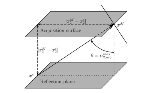
Next, the influence of the acquisition surface and the radiation characteristics are discussed by analyzing the minimum apparent wave speed. The required spatial sampling criterion is obtained by the obtained minimum apparent wave speed in Eq.
Modelling results
Figure 6.7 shows the real and imaginary parts of the acquired image for the multi-component algorithm. In Figure 6.9, the total field expressions are used for the inverse wavefield extrapolation of the multi-component image algorithm.
Testing site
A drainage pipe was present at the bottom of the test site to enable the control of the water level, which can be observed in Figure 7.1. To obtain a homogeneous distribution of the sand at the test site, water was pumped into the closed system.
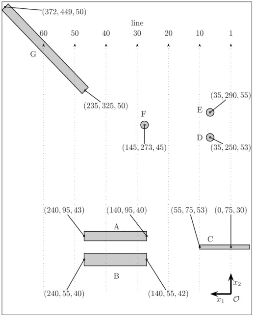
Buried objects
On one side of the test site, an area of 3 by 4 meters is used to perform the measurements. The position of the objects is shown schematically in Figure 7.3, and the properties are given in Table 7.1.
Description of the measurement set-up
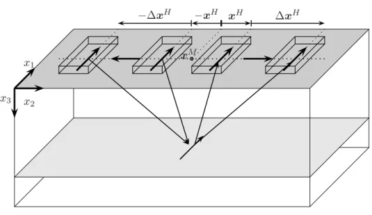
Measurements were made with the pulseEKKO 1000 system using the four inline orientations of the source and receiver antennas shown in Figure 5.2. This frame enables the four inline orientations of the source and receiver antennas as shown in Figure 7.5.
Acquisition parameters
To achieve accurate cross-line positioning, the plastic reference frame was used on which strings were placed at specified positions on each side of the survey line. The temporal sampling interval was 50 ps, which was used to obtain 1000 samples, resulting in a time window of 50 ns.
Pre-processing
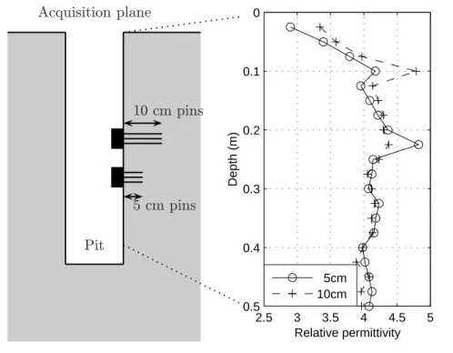
Medium properties
These TDR measurements show that the shallow part of the subsoil has different medium properties compared to the soil that is present deeper in the subsoil due to e.g. This is caused by the influence of the weather on the shallow part of the subsoil.
Three-dimensional imaging results
Equi-amplitude surfaces for the multi-component imag-
Since the imaged contrast of the different objects had different maximum amplitudes, different thresholds were used. Note that the equal-amplitude results are only shown to provide a general idea of the various objects present at the test site.
Comparison between the imaging algorithms in differ-
To enable a comparison, the results of the different imaging algorithms are normalized with respect to the absolute maximum value obtained for the multicomponent image result. These artifacts are not as apparent in the image results shown in Figure 7.12 for the multicomponent algorithm, where the absolute values of image contrast are plotted.