Kazakov, I declare that this thesis entitled "Computer simulation methods of soft matter" and the work presented in it are mine. The study provides a comparison of the new method with pure coarse-grained and mean-field methods.
Motivation
Computer Simulations
At this model resolution, it is now possible to study local motions (eg peptide motifs, DNA intercalation, etc.). However, it is possible to further reduce the model resolution and achieve mean-field models.
Polymers
To reach larger length scales, one of the ways is to reduce the accuracy of the model. Such an approach also extends the system development time, as it is done in full-atom simulation models.
Carbon-based materials
Such types of models have shown very good results regarding experiments with reduced computational costs. Thus, it is essential to convert the computational cost to another tile to ensure the uniqueness of the system.
Aims of the study
Outline of thesis
- Linear chain and osmotic pressure
- Branched polymers
- Networks
- Stimuli responsiveness
- Desalination
Polymers can be neutral or carry some charge (polyelectrolytes) and be differently charged depending on the environment or carry both charges (polyampholyte). The branched architecture has a large variety of examples: such as star-like polymer, combs, dendrimers, H-branched, leather, etc. The star-like polymer can be thought of as a set of linear chains connected by one point (see Fig.2.1b).
Carbon-based materials
- Fullerenes and computational complexity
- Machine learning potential
- Velocity-Verlet algorithm
- Ensembles and Ergodic hypothesis
FIGURE 3.4: The overall potential for simple model of single polymer chain with Lennard-Jones and FENE potentials. There are practically too many particles present in the studied system for the analytical solution of the equation of motion.
MC-SCF
Monte Carlo
From the point of view of computer simulation, the only interest of polymer simulation is the achievement of thermodynamic equilibrium. Changes in the case of the fully connected hydrogel-like system was a simple movement of the segment in space.
Scheutjens – Fleer self-consistent field
However, there are ideas of the method that are essential to consider when using the technique. The recalculation of the potential su(⃗)r (for both the polymer segments and the solvent) can be done as follows:. 3.27) The procedure is repeated until convergence (self-consistency).
Density Functional Theory
Slater or Gaussian
There are 2 types of orbitals to describe atomic orbitals: Slater Type Orbitals (STOs) and Gaussian Type Orbitals (GTOs). STOs describe the shape of AOs much better, but the GTOs are much easier to calculate for the machine. Apparently, it is faster to calculate combinations of GTOs and simulate STO, rather than to calculate one STO.
The method is useful for studying large and complex systems, ranging from nanomaterials to biomolecules. The last point makes the method promising for the study of systems in the overlap of different disciplines, such as biology, chemistry and physics.
Artificial Neural Networks
Loss function
The ultimate goal of the training is to minimize the loss function to get the best fit observation. During training, the candidate model adjusts its weights and threshold using the loss function as a "guide" to reach the convergence point. Typically, the matching process uses gradient descent, which allows the candidate to determine the direction of the convergence point.
With each training epoch, the candidate parameters are adjusted to gradually approach the minimum.
Types of neural networks
It should be noted that although NNs are called MLPs, NNs are actually composed of sigmoid neurons, not perceptrons. It is made by sequentially stacking hidden layers one on top of the other. A star polymer is a class of polymer architectures that has the simplest topology, but is not trivial.
Even neutral (uncharged) star polymers show promising effects such as swelling or collapsing under different solvent quality conditions. Thus, all these advantages make star polymers a workhorse for testing and cross-validating the MC-SCF method.
Summary of results
Each arm of polymer can be chemically modified and as a result such a structure can provide advantages in various technologies such as agro-industries, biotech industries and et cetera. Unlike the simple chains of polymer, these effects are much more pronounced due to its architecture.
Model
- Coarse-grained model
- Mean-field model
- Hybrid model
- Simulation protocols
The task for the MC protocol is to find successive explicit particle positions to sample the positional degrees of freedom of the star's segments. First, we randomly select the explicit node in one of the star arms (the empty segment in Fig.4.2). In the MC-SCF method, the performance does depend on the size of the box size.
More precisely, it depends on the sizes of the MC-SCF fragment (sub-box) and the number of fragments in the star. By selecting one explicit segment, we select (in pivot motion) only one arm of the star.
Results and discussion
- Data analysis
- Center-to-end distance, R 2 ce
- Radius of gyration, R 2 g
- Polymer density profile
- Efficiency
In Fig.4.6a dependences of the radius of gyration are shown as a function of the number of monomers per armN for the MD, the MC-SCF and the 1D-SCF methods at the good solvent conditions. Average values of the radius of gyrationR2 for the MC-SCF and the 1D-SCF methods remain. The number of explicit segments in the MC-SCF method (green curve) can be calculated by (f N/n) +1, where f =3,n=20.
The number of explicit segments in the MC-SCF method (green curve) is 25, for the MC-SCF method with a small number of explicit segments (pink curve) is 7. The MC-SCF (both) and MD methods are in good mutual agreement for all er values.
Conclusion
A polymer hydrogel is a network of cross-linked polymer chains that swell in aqueous solutions without dissolving. Among water desalination approaches, one of the membrane techniques, namely reverse osmosis (RO), stands out for its simplicity and relatively low operating costs [96, 97].
Summary of results
Models
- Gel model
- Coarse-grained model
- Mean-field model
- Maxwell construction
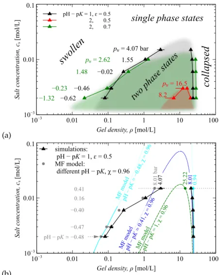
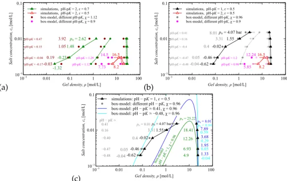
When the pressure is determined, the osmotic pressure of ions is subtracted, whereby the partial pressure of the gel, p,i, is estimated. In such an approximation, a single chain of the gel was considered in a mean field produced by the other components of the system: water, salt ions and the rest of the gel [14]. The entire formula for the free energy is a function of the gel densityφ and contains the parameters χ and pH−pKas.
At this point, the free energy of the system is concave, with two local minima and one local maximum. One of the treatments of the free energy convexity is the Maxwell construction which makes it possible to project the experimental behavior of the system.
Results and discussion
- Pressure extension curve
- Ionization degree and ion transfer
- Phase diagram
- Phase diagram snapshots
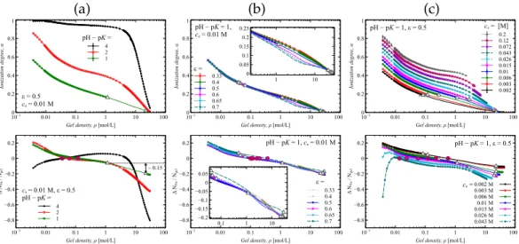
Although the pressure is constant in the two-phase region, the average gel density, φ, varies with compression. As in Fig.5.3a and Fig.5.3b, compression discharges the gel, but the salt concentration significantly affects the ionization rate of the gel. The higher the salt concentration, the higher the degree of ionization of the gel.
From the point of view of desalination, we took into account the change in the number of Na+ ions (see the second line in Figure 5.3), because they are the counterions of the hydrogel. FIGURE 5.3: The gel ionization rate α and the change in the number of Na+ ions in the volume V0, normalized by the number of gel segments N is a function of the gel density φ for different (a) pH−pK, (b) solvent quality ε, and (c) salt concentrations.
Conclusion
Summary of results
Model and Method
Neural network training and testing
Here we follow the approach of Schüttet al.[116] which uses convolutional NNs and only briefly mentions the main points of the whole process in Fig.6.3. Molecular quantities (energies, forces, dipole moments) on NN output are calculated from atomic contributions. The atomic coordinates on NN input are first made invariant with respect to translations and rotations through the use of symmetry functions [64].
We use a convolutional NN with 5 hidden layers for energy and forces and 4 hidden layers for dipole moments. The loss weights are set up empirically to account for different scales of energy, forces and dipole moments.
Results and discussion
NN training results
FIGURE 6.5: Change in predicted force and DFT per atom as a function of the number of carbon atoms for the unperturbed data set s = 0. In addition to energies and atomic forces, dipole moments were also trained, as can be seen in Figure 6.6, where the Cartesian components of pNN−pDFT are shown. FIGURE 6.6: Difference between predicted and DFT dipole moment per atom for the unperturbed s = 0 data set.
For the complete picture of NN training, it is also good to mention the statistics for disturbed structures as well. The statistics for nons = 0 structures energyEℓ, forceFℓand dipole momentDℓlosses are presented in Table 6.1.
Energy minimization
Comparison with GAP-20
FIGURE 6.8: A comparison of energy (a) and force (b) predictions between our GAP-20 (empty box) and NN (solid box) for the same DFT configuration with the appropriate reference point (Ih-C60), which was the same configuration but the calculated energy value was calculated. A similar trend can also be seen in the comparison of forces shown in Fig.6.8b, where our NN is more accurate since the forces are included in the model. Figures/snaps/data/splitted/render/20_A-tga-converted-to.jpg./Figures/snaps/data/splitted/render/20_A-tga-converted-to.jpg./Figures/snaps/data/splitted/render/20_A-tgaure-splitted.jpg/Figures/snaps/data/splitted/render/20_A-tga-converted-to.jpg./Figures/snaps/data/ splitted/render/20_A-tgaure. /20_A-tga-converted-to.jpg.
Conclusion
At the beginning of this thesis, star-like polymers were discussed using different resolution scales: mean-field, coarse-grained and hybrid representations. In the middle of the thesis, the hydrogel under poor solvent conditions was the focus of the story. The molecular dynamics simulation showed the phase transition of the hydrogel under specific external stimuli.
Precisely, the phase transition can be extended by decreasing the pH-pK difference and/or decreasing the solvent quality. At the end of the thesis, the density function theory and the machine learning routine were discussed.