Study of production of jets and dijets in Xe+Xe and Pb+Pb collisions at the

121/2000 Sb., Copyright Law, as amended, specifically that Charles University has the right to enter into a license agreement for the use of this work as a school work in accordance with Article 60 subsection 1 of the Copyright Law. Self-normalized distributions were measured in dijet asymmetry measurements [14, 15] and they allow to quantify the influence of jet damping on the dijet moment balance in the simplest way.

Quantum Chromodynamics

The model has a local SU(3)×SU(2)×U(1) gauge symmetry that gives rise to three fundamental interactions. The SU(2)×U(1) symmetry is responsible for the electroweak interaction, the unification of the weak and electromagnetic interactions.

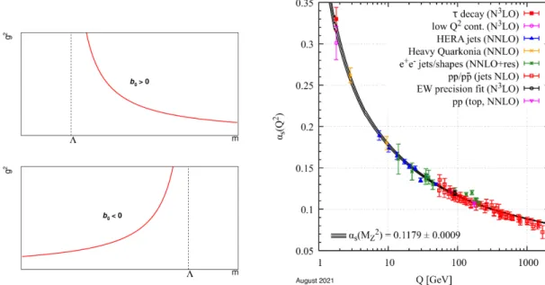
Running Coupling Constant

To choose µclose to the scale of the momentum transfer Qin a given process, then αS(µ2 =Q2) is an indication of the effective strength of the strong interaction in that process [23]. For this reason, a perturbative QCD cannot be used in describing the structure of baryons or mesons.

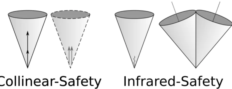
Figure 1.2: Left: Landau poles for two signs of parameter b 0 . Right: A summary of different measurements of α S for different energy scales Q

Jets and Jet Algorithms

Jet Alorithms

This is only partially correct - the input can be many different objects, for example, charged particle tracks, calorimetric clusters, and particles as well. Integrating over all possible values of s, the nuclear thickness function TAB(b): is obtained. 2.3) The product TAB(b)σinelNN, where σinelNN is the cross section of the nucleon-nucleon inelastic distribution, gives the nucleon-nucleon interaction probability.

Figure 1.3: A demonstration of unstable behavior of jet algorithms. Left: Colin- Colin-ear unstable

Centrality of Collision

The number of participating nucleons Npart is monotonically proportional to the energy deposited in the front regions of the detector (3.2<|η|<4.9) [16]. Then, we can relate the geometric quantities to the same central intervals between the data and the MC.

Jet Quenching

The mass of the quark that initiated the jet may also play a role in the suppression. The position of the vertex and the non-circular shape of the overlap result in different path lengths in the medium.

Figure 2.6: Left: Highly asymmetric event with one jet with p T > 100 GeV, but no evident recoil jet

Dijet Balance Measurements

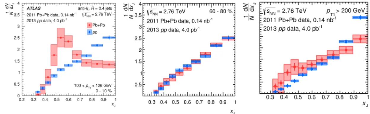
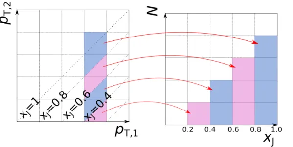
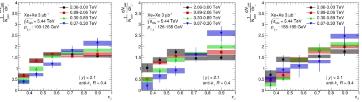
That is, the expansion of the xJ distributions is increasing with increasing centrality and decreasingpT,1. Right: Absolute normalized xJ distribution for pp collisions and five Pb+Pb centrality intervals for the 100 < pT.1 <112 GeV interval.

Figure 2.13: A cartoon of a dijet used in Ref. [14, 15] and Xe+Xe analysis pre- pre-sented in Chapter 5

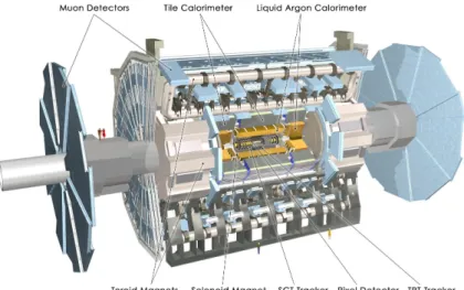
The ATLAS Detector

The Magnet System
Inner Detector
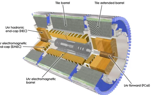
Calorimeters
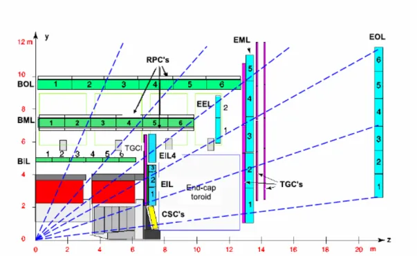
Muon Spectrometer
Zero Degree Calorimeter
ATLAS Triggers and Data Acquisition

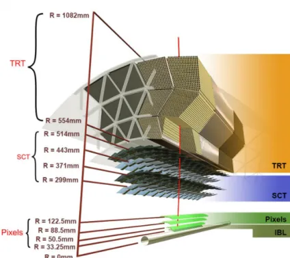
Since this detector is in front of the calorimeter systems, minimization of particle interaction was required. Two end pieces consisting of three discs each are installed on both sides of the detector. The other parts of the detector have a coarser granularity, however sufficient for the necessary radiation and ETmiss measurements.

The LAr forward calorimeter (FCal) covers the most forward regions of the calorimetric system for η values between 1.5 and 4.9. The Zero Degree Calorimeter (ZDC) [83] consists of a sampling calorimeter located 140 m from the IP symmetrically on both sides of the detector. The first level is called the Level-1 trigger (L1) and is implemented in the detector's hardware.

Figure 3.3: Cut-away of the ATLAS detector with its main parts: The Inner Detector, Calorimeters, Muon spectrometer, and magnet systems

Numerical Inversion

Theρ3, νn3 and Ψ3nn from the last iteration are then used to subtract the UE from all beam planes.

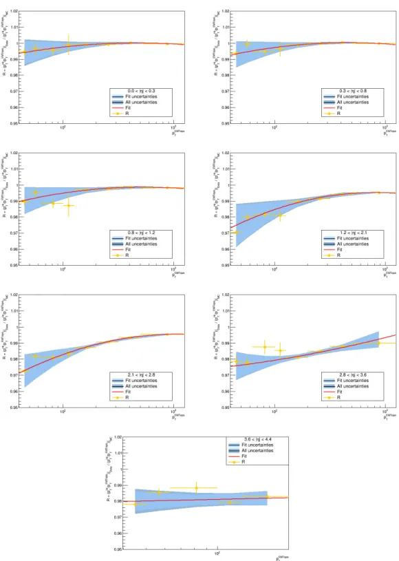
Cross-Calibration

Statistical uncertainties are represented by error bars and systematic uncertainties are represented by the blue band.

Jet Performance

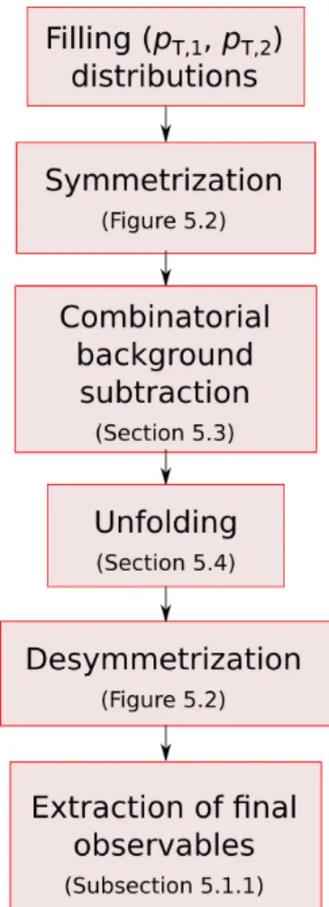
Extraction of Observables

The ratio of a pair of nuclear modification factors between Xe+Xe and Pb+Pb collisions — ρXe,Pb. A comparison of the xJ distributions measured in Xe+Xe and Pb+Pb revealed a difference, as we will show in detail in Section 5.6. This difference can be partly attributed to the difference in the cross section of the hard process due to the different energy of the center of mass between Xe+Xe and Pb+Pb collisions.

The ratio of a pair of nuclear modification factors between Pb+Pb and Xe+Xe — ρXe,Pb. Since pp data are not available for 5.44 TeV, reference pp data at 5.02 TeV, which were used in the Pb+Pb analysis, are used instead. At the same time, ρXe,Pb can be interpreted as a simple ratio of yields, where the yields measured in Pb+Pb are corrected for the difference in the energy of the center of mass of the cross section that describes the hard process.

Figure 5.3: Cartoon depicting slicing of the (p T,1 , p T,2 ) distributions and projec- projec-tion of the bins into x J distribution.

Monte Carlo and Data Events

Centrality Definition

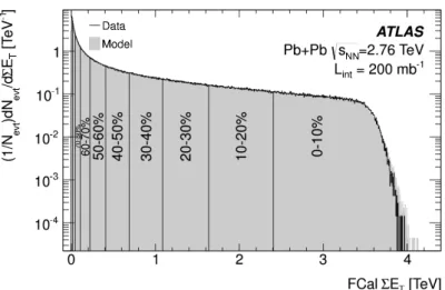
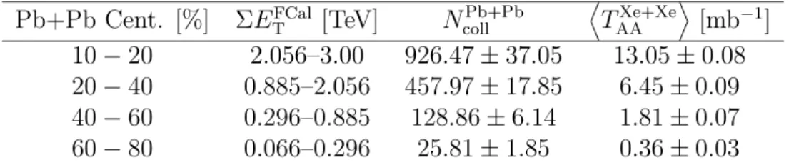
Of course, this correction does not correct all differences between Xe+Xe and Pb+Pb, namely the impact of nPDFs, the impact of the geometry difference, etc. The ΣETFCal distribution is distributed in percentiles of the total inelastic cross section for Pb+Pb collisions. The first percentile, 0-10%, represents the 10% of collisions with the greatest event activity and the smallest impact parameter.

The ΣETFCal distribution with the corresponding quantiles is shown in Figure 5.6, overlaid with the 2015 Pb+Pb distribution as the two collision systems are compared in this analysis. The Xe+Xe results are also compared with Pb+Pb results in Pb+Pb centralities. That is, we take Pb+Pb centrality intervals and apply their ΣETFCal bounds to Xe+Xe collisions.

Event Selection of Xe+Xe Data

The last percentile, 90−100%, represents the 10% of collisions with the smallest event activity and the largest impact parameter. Additional event cleaning to remove additional detector errors (problematic events due to LAr, Tile, SCT, incomplete events) using standard AT-LAS methods. The cut to remove a small number of pileup events is done through a simple cut based on a close correlation between ΣETFCal and the number of reconstructed tracks.

This correlation is shown in Figure 5.7 along with a line representing the cut where everything below the line is rejected. The right panel of Figure 5.7 shows the fraction of events without pileup after the rejection has been applied and indicates that the fraction of removed events is very small for the majority of ΣETFCal values.

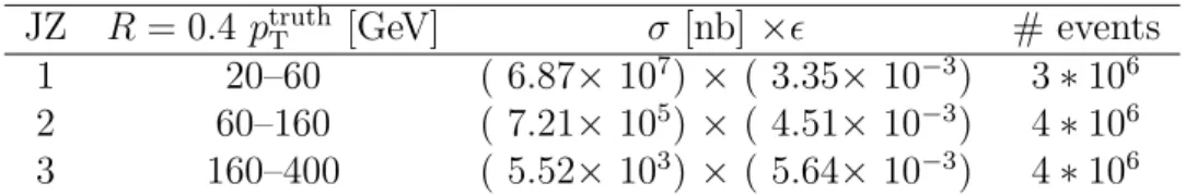
Table 5.1: Centrality ranges for Xe+Xe collisions used in the analysis with their corresponding ΣE T FCal , N coll Xe+Xe , and ⟨︂ T AA Xe+Xe ⟩︂ values

Monte Carlo Samples

The table shows the MC generator level jetspTranges (ptruthT ), cross sections (σ), filtering efficiency (ϵ) and number of events for JZ slices. For ΣETFCal ≳3 TeV, the ratio is subject to very high fluctuations resulting from low statistics. The constant was chosen as a value of the last bin used by the distribution before fluctuations were present.

Over 99.9% of both data and MC events are below ΣETFCal <3 TeV — therefore this simple removal of the fluctuations is a sufficient replacement. Right: The ratio of Xe+Xe data to PYTHIA8 MC — the blue line represents the ratio and the red line is the ratio corrected for statistical fluctuations. Another MC generator — HERWIG7 was used to generate events with the same setting as PYTHIA8.

Table 5.3: PYTHIA8 MC generator samples used in the Xe+Xe dijet balance analysis. The table shows MC generator-level jets p T ranges (p truth T ), cross-sections (σ), filtering efficiencies (ϵ), and number of events per JZ slice.

Combinatorial Background

Background Subtraction

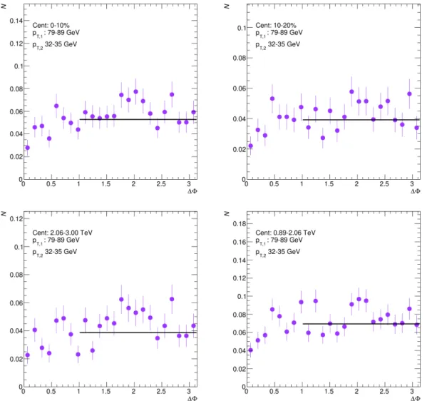
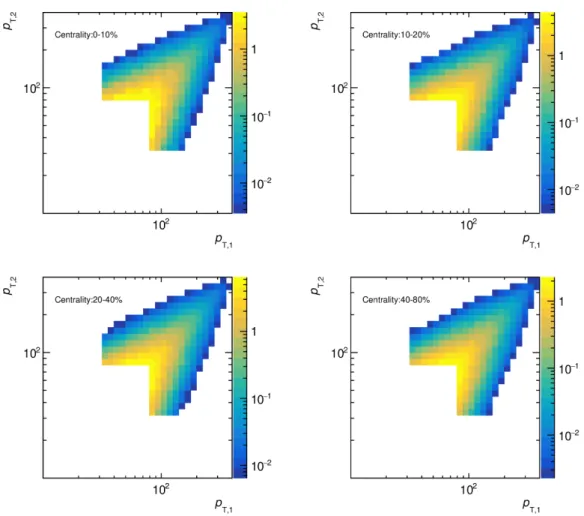
The absolute magnitude of the background compared to the signal in the Xe+Xe collisions is shown in Figure 5.12 - here the (pT,1, pT,2) distribution is plotted on the pT,2 axis and the four pT,1 bins with the most dominant background are shown. The background subtraction correction is largest in the most central collisions and at low pT where it reaches 18%. In the other center bins, the background contribution is less than 3% for all pT,1 and pT,2 bins.

The background magnitude compared to the signal in MCPYTHIA8 is shown in Figure 5.12 — here the (pT,1, pT,2) distribution is projected onto the pT,2 axis, and four pT,1 bins with the most dominant background are shown. The relative magnitude of combinatorial background to signal in Xe+Xe collisions in 0–10% centrality interval is shown in Figure 5.13. Distributions are evaluated for four centrality intervals and for the lowest pT,1 selection, where the background is most important.

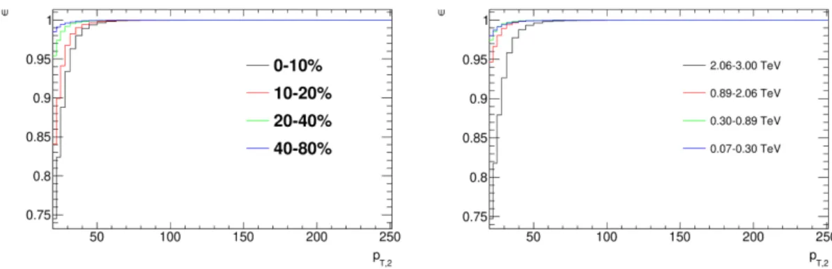
Figure 5.10: Distribution of combinatorial dijets in MC PYTHIA8 at √

Efficiency Correction

Blue — close-up of the unmatched reconstructed jets; green — closing to the background subtraction; purple — closure after background subtraction and the efficiency correction.

Unfolding

Response Matrix
Reweighting the Response Matrix
Statistical Uncertainties
Selecting the Number of Iterations
MC Closure Test
Refolding of MC and Data

Smearing the reconstructed 2D histogram 100 times and then unfolding each smeared version separately with the nominal response matrix. Smearing the response matrix 100 times and using it to expand the nominally reconstructed (pT,1, pT,2) histogram. In general, the magnitude of statistical uncertainty due to the statistical inaccuracy of the reconstructed data is greater than that due to the response matrix.

Green and blue lines represent components of the statistical uncertainty of the smearing histogram and response matrix, respectively, and the black line is their quadrature sum. Here, half of the events from the MC are used to fill the response matrix and the other half to fill the (pT,1, pT,2) measured distribution. The bottom part, then, is their closure, which is defined as a ratio of the two.

Figure 5.16: Underlying measured distributions from the response matrix in four centralities in PYTHIA8.

Systematic Uncertainties

Systematic Uncertainty on the x J Distribution

The above systematic uncertainties were calculated for the xJ distribution, and the results for pairwise normalized xJ distributions for all centrality and pT bins are presented in Figure 5.27. Systematic uncertainties for pairwise normalizedxJdistributions in ΣETFCal intervals, absolute normalizedxJdistribution in centrality intervals, and absolute normalizedxJdistributions in ΣETFCalinterval-. There is no difference between the pairwise and absolutely normalized xJ distributions, except that the absolutely normalized have an additional uncertainty about TAA.

Systematic uncertainties are dominated by JES+JER and prior sensitivity uncertainties in all pT,1 and center bins. The high values of the relative uncertainties in the low xJ bins are caused by the low yields in these bins, where a small change in the absolute yields will cause a high relative difference.

Systematic Uncertainty on the ρ Xe,Pb Ratio

Results

The distributions measured within the same event activity interval are consistent between Xe+Xe and Pb+Pb collisions. The ρXe,Pb(pT,1) and ρXe,Pb(pT,2) evaluated in the same Xe+Xe and Pb+Pb centrality intervals are shown in Figure 5.36. The results are compared with the already published measurement of dijets in Pb+Pb collisions at.

ATLAS Collaboration, Measurements of azimuthal anisotropies of jet production in Pb+Pb collisions at. ATLAS collaboration, Measurements of the suppression and correlations of dijets in Pb+Pb collisions at 5.02 TeV, arXiv Accepted by Physical Review C. Medium-induced modification of Z-tagged charged particle yields in Pb+Pb collisions at 5.02 TeV with the ATLAS detector.

Nuclear modification factor measurement for charm and bottom hadron muons in Pb+Pb collisions at 5.02 TeV with the ATLAS detector. 65] Measurement of substructure-dependent beam suppression in Pb+Pb collisions at 5.02 TeV with the ATLAS detector.