To approach this goal, the estimation of both, aleatory and epistemic uncertainty in the context of dense stereo matching is addressed in this thesis. As in many other fields, the introduction of deep learning in dense stereo matching has brought a significant improvement in accuracy.
Problem Statement
What assumptions and simplifications must be made in order to be able to train such a network. How are the quality of depth estimates and predicted uncertainties affected, and are there any trade-offs between the two to investigate or balance.
Contributions
What possibilities exist to quantify epistemic uncertainty, and are BNNs a reasonable choice given both theoretical and practical aspects? The resulting approach makes it possible to jointly estimate depth as well as aleatory and epistemic uncertainty.
Thesis Outline
The concepts presented in the thesis correspond to the field of uncertainty quantification in the context of dense stereo matching and are based on techniques from the field of deep learning. Section 2.2 briefly introduces the field of uncertainty quantification, focusing on the distinction between aleatory and epistemic uncertainty and their interpretation in the context of dense stereo matching.
Dense Stereo Matching
Terminology and Practical Simplifications
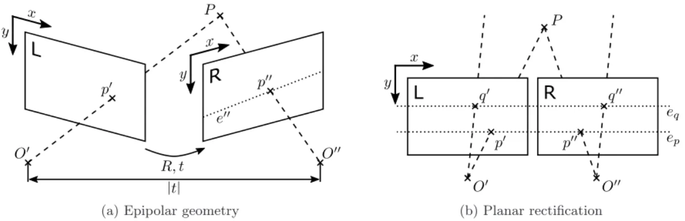
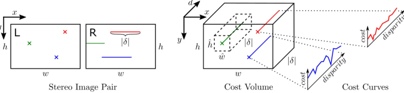
A planar correction further simplifies the matching procedure because all epipolar lines are parallel and horizontal so that the corresponding points are placed on the same image row in both images. Such a disparity allows conclusions to be drawn about the distance between the common plane of the reference image and the matching image and the corresponding 3D point in the model coordinate system.
Taxonomy of the Matching Process
In the first step, the cost calculation, the inequality for possible matches is determined. In the final step of the taxonomy, an established disparity map is refined by applying post-processing techniques.
Challenges and Common Assumptions
By considering such additional information in the definition of the aggregation scheme, it is possible to reduce unwanted smoothing, for example at depth discontinuities. This process means that every point visible in one image also exists in the other image, and requires that such correspondences can be unambiguously identified.
Uncertainty Quantification
In contrast, epistemic uncertainty accounts for assumptions that simplify the matching process, such as those discussed in Section 2.1.3, and features that are missing from the definition of this process (or in the case of deep learning approaches in training). data), such as features and hues that imply a certain geometric shape. Note that the assignment of specific effects to aleatory or epistemic uncertainty is not fixed, but depends on the definition of the problem domain.
Deep Learning
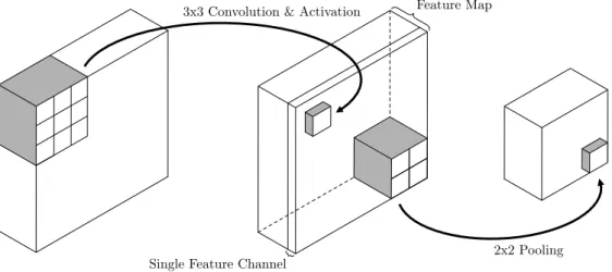
Convolutional Neural Networks
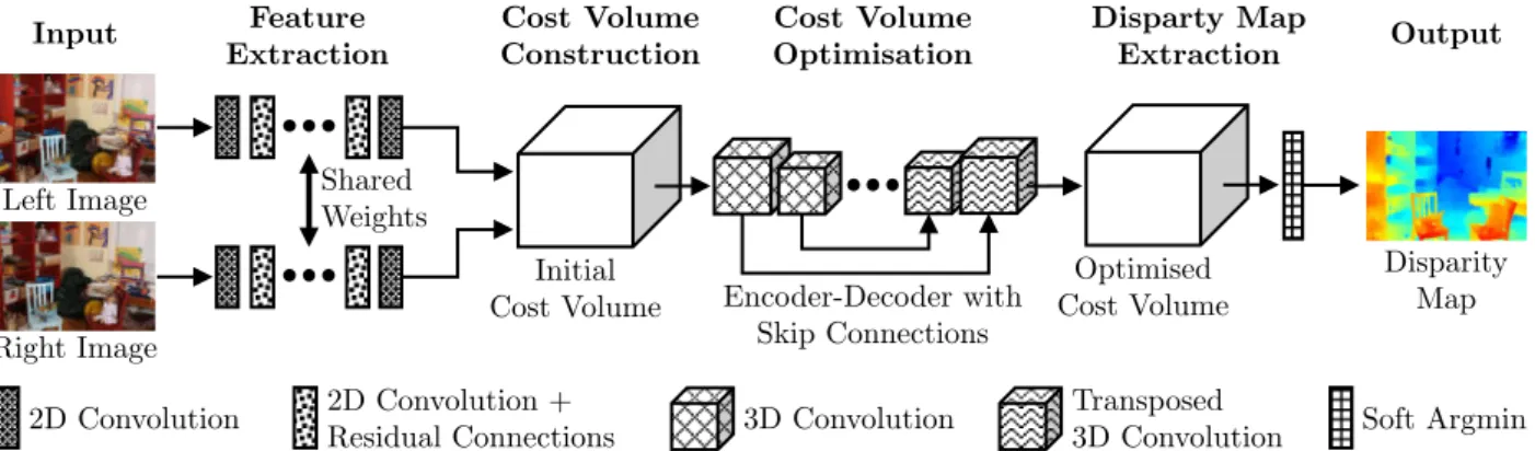
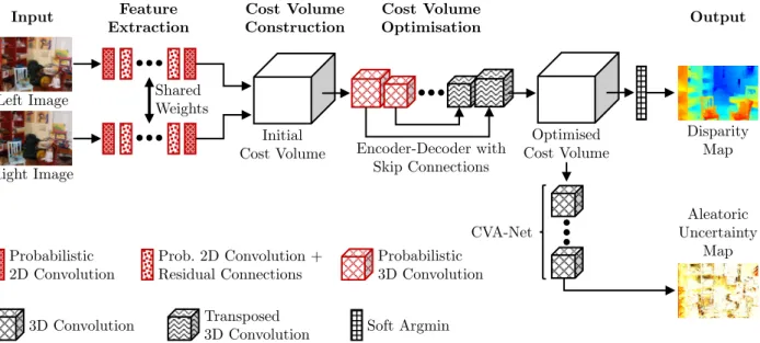
Due to the step of 2 in the first layer of the network, the resulting 4D volume has a spatial resolution equal to 12 of the input images. In the decoder, the spatial resolution is doubled while the number of feature channels is halved with each transposed convolution layer, until the extent of the resulting feature map equals the one of the initial cost volume.
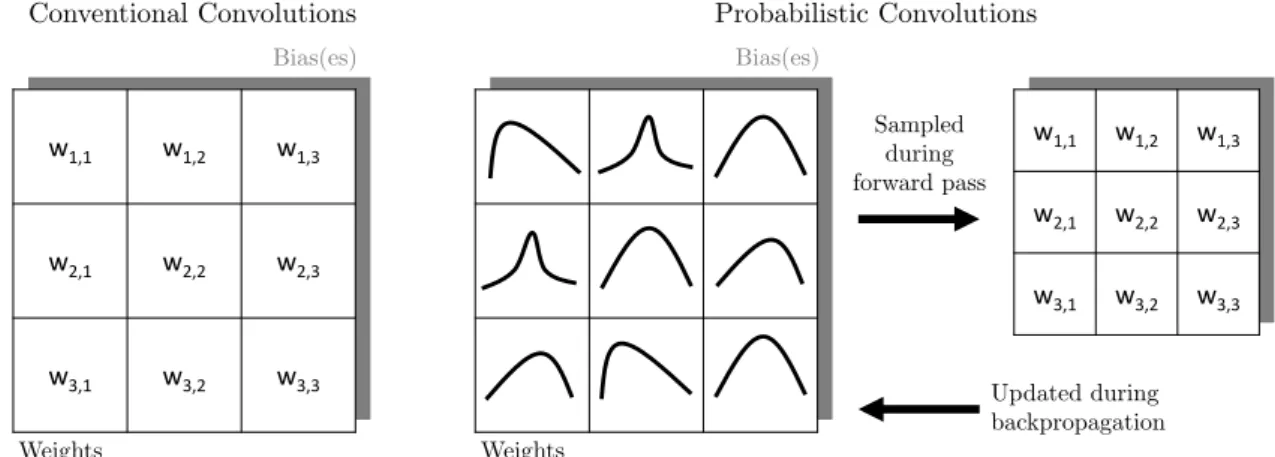
Bayesian Neural Networks
Justified by these advantages, the architecture of GC-Net serves as functional model of the BNN developed in the context of this thesis presented in Section 4.3. To overcome this problem, the exact posterior distribution is usually approximated by bypassing the calculation of the evidence, for example via Markov Chain Monte Carlo (MCMC) approaches (Geyer, 2011) or by using VI (Blei et al., 2017).
Dense Stereo Matching
The approach of Guo et al. 2019) follows a similar idea and combines the information contained in the feature vectors into groups. Based on the concept of the PatchMatch algorithm (Bleyer et al., 2011), the RNN is trained to iteratively select random mismatch proposals that propagate locally.
Aleatoric Uncertainty Estimation
As a result, additional information about the appearance of the scene can be taken into account in the uncertainty estimation procedure. Limiting the information considered in this way leaves this approach vulnerable to noise and cost volume outliers.
Epistemic Uncertainty Estimation
Another realization of the concept of stochastic neural networks is Monte Carlo dropout, which is used for example by Gal and Ghahramani (2016), Kendall et al. To address this issue, Zeng et al. 2020) have recently proposed to treat only some layers of the network in a probabilistic manner, while keeping all others deterministic.
Discussion
To the best of the author's knowledge, close stereomatching has not yet been the subject of research in the context of epistemic uncertainty estimation. In this chapter, a new method is proposed to estimate the aleatory and epistemic uncertainty in the context of close stereo matching.
Overview
This chapter closes with a discussion in section 4.5, addressing the assumptions made in the context of this approach as well as the limitations of the presented methodology. Rather, f(c) together with f(d) are realized as a BNN described in Section 4.3, to jointly estimate inequality and epistemic uncertainty.
Aleatoric Uncertainty Estimation
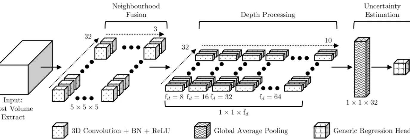
CNN-based Cost Volume Analysis
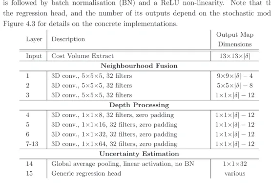
To process complete cost curves, the depth|δ|of an extraction is chosen to be equal to the depth of the cost volume. Furthermore, zero padding is used for all convolutions in the depth processing part of the network.
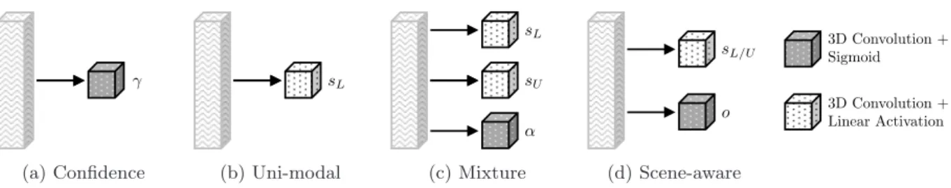
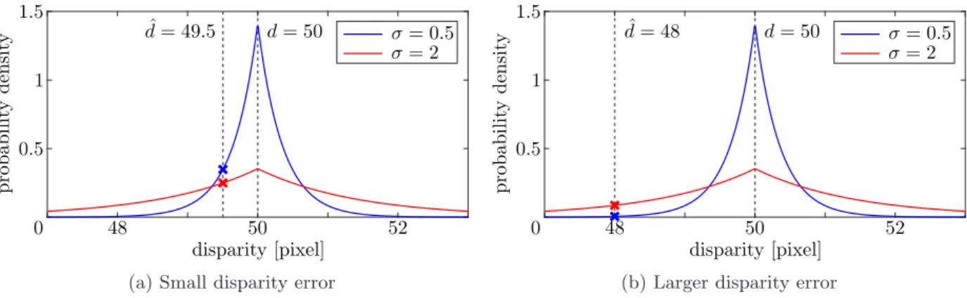
Uncertainty Models
Note that the estimation of aleatory uncertainty is assumed to be independent of the disparity estimation process. With the ratio of the interval length to the standard deviation σU of the uniform distribution, it is further: r.
Epistemic Uncertainty Estimation
Functional Model
In contrast, the parameters belonging to the operations used to upsample the intermediate feature maps (3D transposed convolutions) performed in the decoding part of the cost volume optimization step are kept deterministic (cf. the accuracy of the deterministic version is directly affected when reducing the number of characteristic channels.
Stochastic Model
Furthermore, this adaptation of nc also reduces the size of intermediate feature maps since the feature channel number specifies one of the four dimensions of such a feature map as illustrated in Figure 2.3. In summary, the proposed transformation of the GC-Net architecture into a probabilistic variant using 24 filter channels increases the number of parameters to be learned only slightly from about 2.8 to 2.9 Mio. assuming the stochastic model is defined as described in the next section), reducing the memory footprint of intermediate feature maps by 25%.
Joint Uncertainty Estimation
As a consequence of this integration, the output of the CVA-Net is affected by the stochastic nature of the early stages of the probabilistic GC-Net. More precisely, the estimated aleatoric uncertainty map depends directly on the network parameters randomly drawn from the posterior of the variance distribution.
Discussion
The last part of the presented method deals with the combination of CVA-Net, which is used to estimate aleatoric uncertainty, and the probabilistic variant of GC-Net, which allows jointly estimating inequality and epistemic uncertainty. The assumption of independence of uncertainties is therefore a simplification that requires further investigation.
Objectives
For this purpose, the objectives of the evaluation are introduced in Section 5.1, before the datasets used for training and testing are presented in Section 5.2. What is the contribution of the individual components to this result and how well do these components integrate?
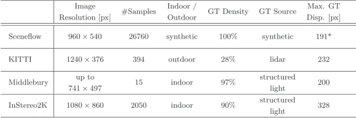
Datasets
Dense and subpixel accurate ground truth disparity maps are obtained with a structured light-based approach. The figure contains an example per dataset, consisting of the reference image and the corresponding ground truth disparity map.
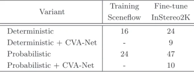
Training and Hyper-parameter Settings
- General Remarks
- CVA-Net
- Probabilistic GC-Net
- Combined Approach
AlsoβBCE is set to one, which weights the binary cross-entropy term equally relative to the probability term in the loss function of the scene-aware variant (see Eq. 4.12). The individual values of β-error are determined based on the error distribution of the training samples using GC-Net without CVA-Net.
Evaluation Strategy and Criteria
- Disparity Error Metrics
- Confidence Error Metric
- Uncertainty Error Metric
- Region Masks
- Monte Carlo Sampling
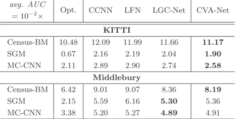
In this context, an ROC curve represents the error rate as a function of the percentage of pixels sampled from a disparity map in order of increasing uncertainty. In this chapter, the results of the experiments performed in the context of this work are presented and analyzed.
![Figure 5.3: Effect of the number of Monte Carlo samples drawn. At test time, an average disparity estimate ¯d is computed based on disparity estimates d k with k ∈ [1, .., K], corresponding to K different Monte Carlo samples (cf](https://thumb-eu.123doks.com/thumbv2/1library_info/19327328.0/82.892.225.648.105.367/figure-disparity-estimate-computed-disparity-estimates-corresponding-different.webp)
CVA-Net Architecture
On the other hand, depth discontinuities, which are also often identified as particularly demanding in the context of dense stereo matching, show one of the limitations of the presented CVA-Net architecture. SGM Discrepancy Score CVA-Net Confidence Map Figure 6.4: Visualization of the problem with SGM-based discordance maps.
Aleatoric Uncertainty Models
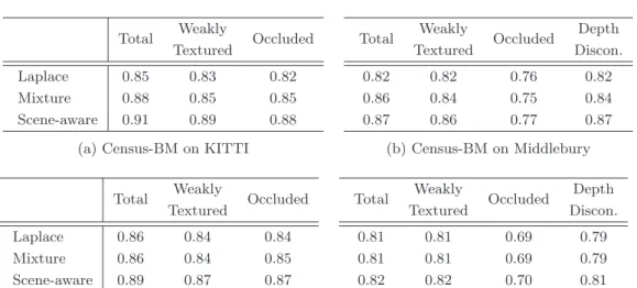
Note that the values of the three uncertainty maps are scaled to the same range to allow an easier comparison. In the definition of the scene-aware model, as presented in this thesis, pixels located close to such depth discontinuities are not treated as belonging to a challenging region, and the associated uncertainty is thus modeled using a Laplace distribution.
Dense Stereo Matching using a Bayesian Neural Network
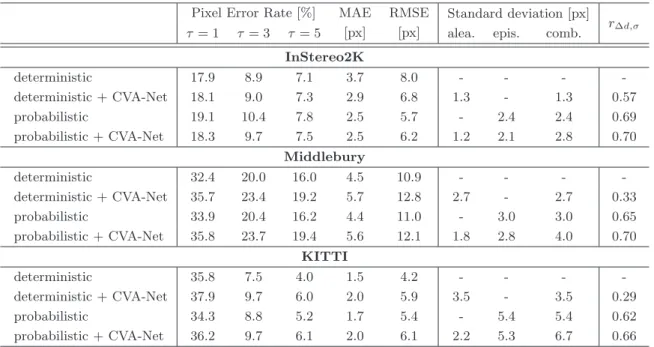
Comparison to the Deterministic Baseline
Consequently, the superior performance of GC-Netprob with respect to poorly textured image regions can be mainly explained by the Monte Carlo sampling approach applied to approximate the disparity prediction distribution. In contrast, the comparison of inference time reveals significant differences and demonstrates a drawback of approaches based on Monte Carlo sampling: While the difference between the deterministic and probabilistic variants using a single Monte Carlo sample is comparable to that in training. time, the completion time increases linearly with the number of samples drawn.
On the Relevance of Aleatoric and Epistemic Uncertainty
Thus, it can be assumed that the quality of the disparity estimates has a direct impact on the ability to estimate the associated aleatoric uncertainty. Despite the remaining open challenges discussed, the consideration of aleatory uncertainty is therefore still useful, also in the context of the highly accurate disparity estimates obtained with GC-Net.
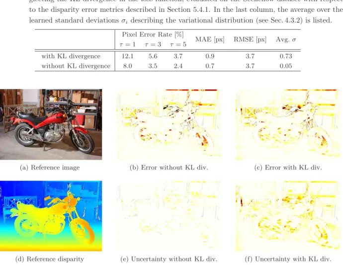
The Kullback-Leibler Divergence and the Mode Collapse Problem
The table shows the results of the probabilistic variant of the proposed GC-Net, considering or neglecting the KL divergence in the loss function, evaluated on the Sceneflow dataset with respect to the disparity error metrics described in section 5.4.1. Evaluated on the test samples of the Sceneflow dataset, the figure illustrates that considering the KL divergence in the optimization objective is essential to obtain well-calibrated uncertainty estimates.
Discussion
In: Proceedings of the International Conference on Medical Imaging and Computer-Assisted Intervention, Springer, Cham, pp. In: Proceedings of the Conference on Neural Information Processing Systems Workshop on Bayesian Deep Learning.