This allows us to compute the cohomology of the space Ym,n(σ) from the cohomologies of the spaces Ym,n−1(τ) from which it is constructed. We start by showing that they are homotopically equivalent to the loop space Ω(SUm/Tm−1), which gives us the cohomology of the boundary space.
Loop spaces
By [Mil63, Theorem 17.1], this is homotopy equivalent to the space of piecewise smooth loops inX, and we will usually work with this space instead. This shows that all such spaces are homotopy equivalent, so we will not make a big distinction between them.
Flags
We will only be concerned with the case where X is a Riemannian manifold, so it comes equipped with a Riemannian metric g and an induced topological metric. By defining a cover of X with good properties, we will be able to work exclusively with loops where we have some control over their behavior.
Coxeter groups
The Bruhat order on the Coxeter group W with generators S is the transitive closure of the relation. In this chapter, we will introduce the spaces that will be studied in the rest of the document and collect various useful results.
Symmetries
But this means choosing 1inCma after removing a finite number of proper subspaces, since the dimensions of the spaces on the right arem−1 for Vm−1andm−n for all the rest. While all of these symmetries are fun to work with, the spaces as defined above have some problems.
Stabilisation
But this space is the same as Ym because the right flag of the lower triangular matrix and the left flag of the upper triangular matrix are equal to the corresponding flag of the identity matrix, as we saw in Section 1.3. Since the above is done by matrix multiplication, it commutes with the torus action Tn on Ym,n and everything can be repeated with Ym,n and Ym,n+1. All entries below are null. A, B, C and D are matrices consisting of the corresponding rows from (σ1, .
So we only need to count the number of inversions of each of the permutations, and see that ϕ(I, σ) has fewer inversions than ϕ(J, σ). We now consider pairs (a, b) which are inversions for τ but not for φ, and in which exactly one of the two numbers is in the set. A summary of the statement above is that the mapϕ(·, σ) is order-reversible when we order the indexing sets by inclusion.
Shifting a column to the left is the same as multiplying by, which corresponds to adding all the entries above a given entry.
The limit space
Quaternionic and real cases
We will introduce the spectral sequence that computes the cohomology of Ym,n, and use it to compute the first cohomology groups of all the spaces. Then we focus on Y3,3 and give a complete description of the cohomology, which also leads to the cohomology of the quotient, X3,3. The general method to calculate the homology and cohomology of Ym,n is by using the spectral order of this filtration, as described in Theorem 2.
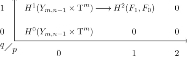
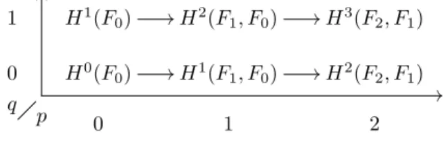
To use the spectral sequence, we need to calculate the cohomology of the pair (Fp, Fp−1). Since Ym,nis is open, we can obtain an open set in Fp by inserting a small plate on these zero entries. The intersection of Ym,n×Dp and Fp−1 corresponds to removing 0 from disk, since one of the entries inserted in the last column must be non-zero.
This means that the disjoint union of all these forms an open set in Fp with.
The first cohomology of X m,n
THE FIRST COHOMOLOGY OF Xm,n 35 and then insert the coordinate from (D−0) on the ith coordinate in the last column. The second map consists of the differentials from the long exact sequences of the pairs. Ifi6=j, the inclusion will not touch the jth coordinate of Tm, so on cohomology classes it will mapαj to an element that is of the form.
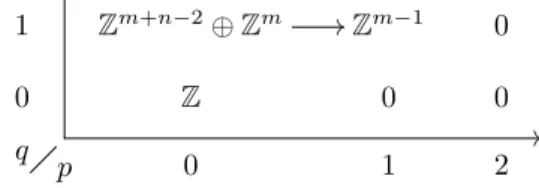
Since the groups involved are all free, we know that the core is also free and we can calculate the rank as the rank of the domain minus the rank of the codomain, which gives us. But by the previous theorem, f∗ is a map between free abelian groups of the same rank, so it must also be injective and thus an isomorphism with inverse Det∗. This shows that the determinant map is an isomorphism on the first cohomology groups and extends immediately to the quotient spaces, with .
So if the class di ∈H1(Ym,n+1) represents the image of moving once around zero in the i'th coordinate of Tn+1, then.
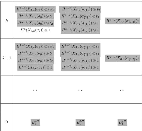
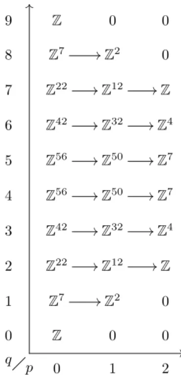
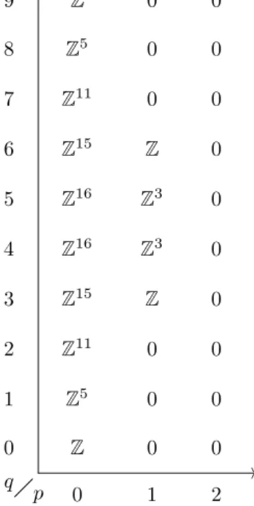
The spectral sequence of Y 3,3
Some of the calculations were done in Sage and the corresponding source code can be found in Appendix A. In Y{1} we have the first entry of the last column equal to zero, which is a space. The space consists of elements in Y3,3 where all entries of the last vector are nonzero.
If the first function is zero, then at least one of the other two must be non-zero. By the implicit function theorem, the coordinate that has non-zero derivative can be written as a smooth function of the other coordinates. Consider a subbundleN R∼=R×D of the normal bundle of R in the tangent bundle T Z, such that the exponential map is a diffeomorphism onN R.
In order to obtain the E2-side of the spectral sequence, we must calculate the homology of the differentials.
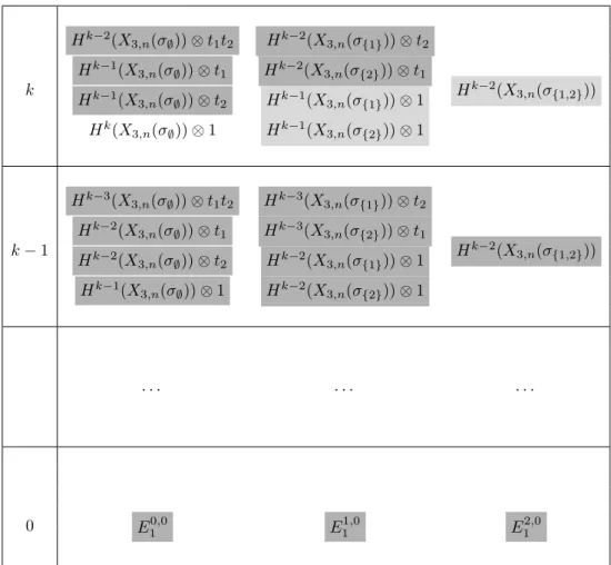
Differentials on E 1
Since we are working with a disjoint union, we only need to calculate inclusion on each factor. In degree 1, this is calculated by dualizing to homology, printing the map onto generators, and figuring out what they map to. To check the sign, we need to check if this map preserves the orientation of the torus in R.
If we use the pair homeomorphism at the bottom of the diagram, the limit map at the bottom becomes the sum of two limit maps. Boundary maps are given by a long exact sequence of the pair (D, D−0), so we only need to consider the inclusion on the left. Again, we compute the cohomology map by dualizing to homology and working with dual generators.
We have now reduced everything to computing some known boundary maps for the pair (D, D−0).
Turning the page
We want to show that the boundary space Xm,∞ is equivalent to the space of loops in the flag manifold GLm(C)/Bm. As before, we will start by considering Ym,n and then quotient with the torus Tn. Note that this function descends into the quotient space Xm,n=Ym,n/Tn, since elements Ym,n that are equivalent under the action Tn give paths in GLm(C) that are equivalent under the action Bm.
We want to show that the stabilization map s:Xm,n→Xm,n+1. does not affect mapf, or more precisely that f induces a well-defined map on Xm,∞. To do this, we will work with the subsequence Xm,nm and the sequence Xm,n, since the two limits are isomorphic. This is done by showing that the map sm is homotopy to the map set that inserts the identity on the last columns of A∈Xm,nm,. Since T is an upper triangular matrix, it can be homotoped to the identity without affecting the linear independence of the columns, and the maps are therefore homotopic.
The compound f ◦se is the same as f, except that the loop f ◦es dwells on the identity for a while before terminating.
Homotopy equivalence
The lemma above shows that the images ϕk fit together to define an image from Ω to Xm,∞. The idea is to use the images ϕk as homotopy inverses of the loop space mapf. We want to show that we can construct a map from W to Xm,∞ such that the compositional ◦eg is homotope tog.
But by our choice of ε, each path is homotopic with the path connecting these points with minimal geodesics, so ◦eg'g. The mapf◦g is null homotopic in Ω and the image of the homotopy is compact, so it is contained in Ωk for somek. So the mapg can be stabilized to a null homotopic image, so it must be null homotopic in Xm,∞.
The Pontrjagin homologization of the loop space, with product given by loop concatenation, was calculated in [GT10, Theorem 4.1].
Other coefficients
Other stabilisations
Instead of reducing all the way down to what would correspond to X3,n−1(τ), as we often did in the finite-dimensional case, in this case it is simpler to use the torus action itself to change all non-zero entries in the last column to ones and avoid multiplying by a lower triangular matrix. But the inclusions in X3,∞(Id) are homotopic equivalences, since they correspond to treating a path with a different endpoint in the loop formulation, and we know that they are all equivalent. But using this we can calculate the other side and see that it is concentrated as R⊗1 in the first column as we want.
Cohomological stability
The top row is correct, as it is part of the spectral sequence for X3,∞(σ) and this collapses to the second page by Theorem 33. If we go to the second page of the spectral sequence, we can see that in the row the groups will no longer change. We still know that the cohomology group iX3,∞ is the inverse limit of the cohomology groups ofX3, and that the map L∗ is the projection.
In degree one we get the elementsx1andx2, and in degree two we get 1andx1x2as generators in the homology of the loop space, which correspond to the proper dimensions of the cohomology groups by the universal coefficient theorem. Similarly, the maps induced from L∗n will also have to behave well on the different columns of the spectral row if the proof is to be transferred without too many changes. Continuing to work with this, and applying some conjectures about the structure of the spectral series, it seems that there is a relation between the cohomology of X3,n and the cohomology of the double suspension Σ2(X3,n−1), when the degree of the cohomology group is greater than n.
This provides different maps that can be used to investigate the cohomology and structure of the spaces. The code below calculates the kernel and image of the first boundary map in the spectral sequence for Y3,3, as described in Section 3.5. The code below calculates the orientation of the intersection points of the inclusion maps, as described in Section 3.4.