Decision and evaluation in non-life insurance mathematics

In article B, we analyze the problem of finding the optimal premium for an insurance company as a function of the amount of the deductible with a fixed amount. The definitions here are similar to those in paper A and, as in the paper, we refer to Foss et al. 2013) for a comprehensive treatment of the topic.

Prelimiaries

• Random sums
• Counting and compound processes
• Renewal equations
• Markov chains and processes
• Markov renewal processes and Markov renewal equations
• Heavy-tailed distributions

Let (Xi)i∈N be a set of random variables, and N be a counting random variable (taking values ​​in N0) independent of the Xi's. A corresponding generalization of the renewal equation is the Markov renewal equation in (1.1) of PaperA, viz.

Introduction

The main contribution of the paper to the establishment of (1.1) is to fill this gap. This together with a number of additional steps then enables the completion of the proof of Theorem A.2 in Section A.6.

Preliminaries and statement of main results

Our main result in this direction, Theorem A.3 below, is an extension to sums of the form Pd. The remainder of the paper is then evidence, supplemented by various results of some independent interest.

Random sums of subexponentials

G is a ∆-subexponential distribution function for allT > 0. i) Assume that zj is directly Riemann integrable and zj(x)/g(x)→0 for allj ∈ E. Note that the minimum takes (or multiplied by a positive constant) will preserve properties as a cat lag and non-increasing.

Random sums of local subexponentials

Random sums with subexponential densities

Proof of Theorem A.2

Preliminaries

• Utility and risk attitudes
• Premium principles
• Deductible
• Reserve models and ruin probabilities
• A short note on stochastic control theory

We distinguish according to the extensiveness of the distribution of the size of claims in the sense of chapter 1.1.6. It is now becoming clear how extensive claims threaten the solvency of the insurance company.

Introduction

For a certain deductible, a change in the premium will have a two-way effect on the movement (and profit) of the insurance company. The same applies to the risk aversion parameter, which will be considered as an i.i.d. result.

Customer’s problem

Due to the forgetting property of the exponential distribution, the client still faces an identical problem every period. Assume that the only risk the customer is concerned about when setting the price is the additional risk S(K) she bears when she does not insure. This motivates the use of other already developed premium calculation principles applied by. customer perspective.

Portfolio characteristics

Stochastic claim frequencies

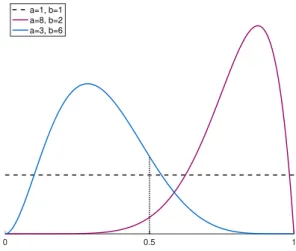
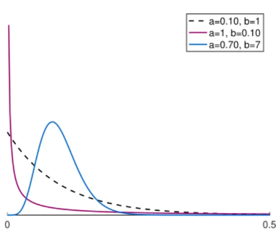
When unobserved heterogeneity in the Bayesian assessment of claim experience is taken into account, the claim frequency is often assumed to be Γ(s, b) distributed, for example as in Pitrebois et al.

Stochastic risk aversions

Ruin probability

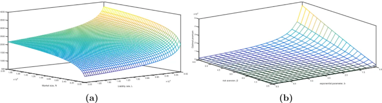
Moreover, due to the obligation rate, L, the spread will also have a negative shift when the premium becomes too high, as no customer will be interested in insuring, so weak→∞µ(p;K ) <0. Conversely, what if the premium was so high that no customer would be interested in insuring. Therefore, if the insurance company sets the premium so high that it is above the reservation price of all N customers, then no customer will insure.

Examples and illustrations

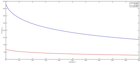
Firstly, the insurer must look at which part of the premium it is profitable to be able to offer insurance. For all considered deductibles in the range [0.5000] the drift will be positive in p(K).˜. The existence criteria of the insurance company are p−αx(K)1 >0, i.e. the premium must simply be greater than the net premium.

I Calculations of the present value in Section 2

If a parameter does not vary, it has the same value as in previous graphs. Again, since the logarithm is an increasing function, one can simply state that the insurance company should choose the maximum of p˜ and p∗.

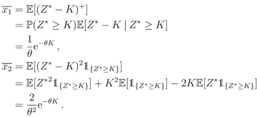
II Calculations of the variance in Section 2

The square of a sum is also used to find the conditional variance in the second term of (B1).

III Illustration of the complexity of the exponential premium in Section 2

Preliminaries

• Terminology of game theory
• Equilibrium types
• A stochastic differential game

If the players' strategies completely determine the outcome, the game is said to be deterministic. In contrast, if a random variable affects at least one of the object functions, the game is called stochastic. A dynamic game is called a differential game if it takes place in continuous time, where a differential equation describing the game's state trajectory is controlled over time by the players' decision processes.

Introduction

This provides an alternative to the approach in the literature on dynamic games in premium controls to assume a demand structure directly, without reference to the customer's problem or market frictions. The characteristics of an individual customer are unknown to the insurance companies, but their probability distribution is known. Thus (3.1) can be considered as a diffusion approach to the Cramér-Lundberg process extended to the case where the insurance companies have access to investment in a risk-free asset.

Customer’s problem

In Section C.2 we analyze the possible criteria for the customer to choose one company over another. Let wi,t be the client's wealth at the moment when it is secured in company i and w0 =wi,0− its initial wealth. If the customer's criterion is to choose the company with the largest value of this quantity, then we arrive at (3.2) again, this time with ρ=r+ 1/ϑ(d−r). 3.4) The client is indifferent if the equality holds, but this case becomes irrelevant in the following as v is taken as random with a continuous typical distribution.

Portfolio sizes

The time horizon T can be the time when the customer expects to need insurance, or the time in which she expects companies to keep premiums relatively constant. With T in Section C.2 being the remaining time the customer needs insurance, T then decreases linearly over time, and so the individual customer will dynamically redo their calculations with the current T (and premiums ). A Bayesian view of allowing customer characteristics (here frictions V ) to vary randomly across customers is quite common in insurance modeling.

The strategies of the insurance companies

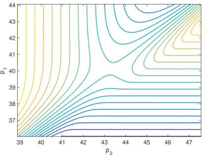
Following Taksar and Zeng (2011), we will only consider Markovian (also called feedback) strategies π, which means that π1(t), π2(t) depend only on the current value δ of the difference ∆π(t) =Rπ1, t−Rπ2,t between the corresponding controlled spare processes Rπ1, Rπ2. The choice of interval(`d, `u) seems arbitrary, but we'll see that later once we've found a Nash equilibrium for a. Solving a Nash equilibrium thus reduces to finding a saddle point of the function ν(p1, p2), with a relative maximum along the first axis and a relative minimum along the second.

The beta case

• Numerical example

Without market frictions, c= 0, or if ρ= 0, premiums are actuarially fair, p∗i =α x1. The higher the cost of frictions or ρ, the greater the deviation from actuarially fair premiums. The contour diagram in Figure 3-5 zooms in on the middle part of the mesh in Figure 3-4 and the saddle point immediately becomes apparent. The distribution of customers across insurers in equilibrium is shown in Figure 3.6, where the cut-off point of (3.6) is v0 = mβ = 0.82.

Conclusion

Each company chooses its strategy to balance revenue per customer against portfolio size, taking into account the strategy of the other company. The reserves of the companies are modeled by means of the diffusion approach to a standard Cramer-Lundberg risk process, extended to allow investment in a risk-free asset. Future research could consider three or more companies competing for market shares, explicitly accounting for the risk of bankruptcy, or for the possibility that some potential customers choose not to insure.

I Second order derivative test in Theorem 11

Introduction

In the literature following Taylor (1986), the individual insurance company is often modeled as determining its premium in response to the total insurance market, without explicitly considering the analogous behavior of the other companies that form this market and the resulting strategic interactions . The claim frequencies of individual customers are considered random for the insurance company, and we obtain explicit solutions for equilibrium premiums in the case of gamma-distributed claim frequencies. In Section D.5 we obtain explicit solutions in the case of gamma-distributed demand frequencies, and provide numerical examples.

Customer’s problem

IfKi 6= Kj, the customer will face an excess claim size risk when insuring with the company with the higher excess. By standard arguments of insurance, because of the risk aversion, the customer will be willing to pay a fee to avoid the additional risk. 2018) we presented a partially more sophisticated approach to the client's problem involving a finite decision horizon with different interpretations, but for the sake of simplicity we did not pursue this aspect here.

Portfolio characteristics

We will take this into account by introducing a personal security load ω(β) that the customer is willing to pay to avoid the excess risk when K1 6=K2. 2018) we have presented a partly more sophisticated approach to the customer's problem involving a limited decision horizon with varying interpretations, but for the sake of simplicity we have not pursued this aspect here. so the portfolio sizes are. 3.7) The average claim frequency for I1 is the conditional expected value of the random claim frequency A given that the customer insures that I1, i.e.

The strategies of the insurance companies

Now consider the resulting drift and variance of the reserves in (3.1), focusing on the case K1 > K2. According to (i) of Lemma D.2, Vπ(δ) has the form S(δ)/S(`u), and the combination of (ii) of the lemma and Note D.1 makes it possible to obtain a Stackelberg equilibrium characterize it with I2 as the leader and I1 the follower. This yields Theorem D.3 below, in which we find the explicit (local) conditions for a Stackelberg equilibrium in (3.11) in terms of the function κ( , ; δ) from (3.15).

Gamma-distributed claim frequencies

• Numerical illustration

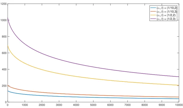
By Proposition D.5, y must be the median of the gamma distribution, that is, the value mΓ that solves. Furthermore, note that by scaling properties of the gamma distribution, mΓ/ai is the mean of a gamma(1, b) distribution. Examples of gamma-distributed claim frequencies across customers are illustrated in Figure 3.1 for different values ​​of parameters a and b.

Conclusions

I Second Order Derivative Tests for Theorem 6

Preliminaries

• The individual’s wealth and objective function
• Pricing by change of measure

In the three previous papers, as part of the analysis, the so-called customer's problem is considered by evaluating the current value E[R∞. Compared to the formulation of the stochastic control problem in Section 2.1.5, this difference in dynamics eliminates the diffusion term of the infinitesimal operator and adds a term related to the jumps of the composite Poisson process, as we see in ( 4.3). Then for three different choices of the price measure function, we compare two cases: one where the individual is limited to a fixed amount deductible structure and one where the individual can freely choose the deductible structure.

Introduction

Aside from appearing in the target function with or without a utility function, the individual's consumption affects individual wealth in the same way that dividends affect the insurance company's risk process. In these types of problems, it is possible for the individual to change strategy more often than the time horizon of the objective. Other publications in this field generally generalize the financial market in which an investment decision is made or the preferences of the individual.

Claims process and insurance contracts

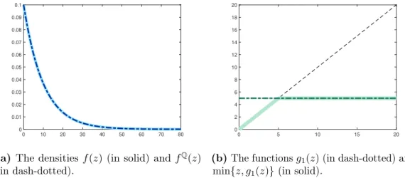
Thus, when choosing an insurance contract gv, the individual's cost is reduced to min{z, gv(z)} depending on the damage. The insured therefore covers the damage min{z, K} himself, and the rest of the damage, namely (z−K)+, is covered by the insurance company. The purchase of insurance then has the following effect on the dynamics of the individual's wealth process.

Optimization problem of the individual

Substituting these optimal values ​​back into the HJB equation (4.5), the supremum is obtained and we can solve for (4.10), verifying that the initial guess for the structure of the value function was correct, since α does not depend on wealth . We will compare the performance of the optimal decisions (c∗, v∗) with alternative decisions, in particular with suboptimal choices of v. Let us denote by V(1) the value function resulting from optimizing (c, v) which gives rise to the coefficient α1 and denote by V(2) the value function resulting from optimizing over c for a given v which gives rise to the coefficient α2.

Pricing by change of measure

In Delbaen and Haezendonk (1989), the variable Zi is the claim to the insurance company from the insured event number i. Let's remember that here Zi is the real loss, while only part of it is claimed from the insurance company. Note that the insurance control in then appears as an endogenous part of the price measurement function.

Insurance products

• Completely flexible
• One level fixed amount deductible

We consider the three choices of the price measure function β introduced at the end of Section 5. The index iβ is reflected in the index of the optimal insurance strategy g∗. Remember that g is unparametrized in this section, so the optimal strategy subscripts g∗ refer to the price measure function and not to the parameterization of g. Once again, we take a closer look at the three price measure function choices.

Numerical illustration

• The impact of the pricing measure function
• The welfare loss

To illustrate the sensitivity to changes in the values ​​of these parameters as clearly as possible, graphs of the relative loss L/ξ are shown in Figure 4.4 for a log-linear pricing. For the log-linear price measure function, β2(z) = log(θ2z+δ2), we see that the relative loss increases as θ2 increases, see Figure 4.4a. Finally, in Figure 4.4d, the relative welfare loss decreases as expected in the loss parameter η.

A digression on power utility

The first-order conditions lead to the optimal choices c∗ andg∗(z), and if we insert these back into the HJB equation and solve, we get α and κ. We note that for the linear pricing rule the optimal deductible is not a constant but a constant fraction of the asset (minus the typically relatively small value of full coverage). For our variance principle, the fraction becomes a linear power function of the loss, and for our Esscher principle, the fraction becomes an exponential power function.

I The impact of pricing on the individual’s decision

A first-order condition on consumption then leads to the same structure as seen earlier, . c∗ =rw− 1 . allogra α. Leibniz's integral rule is used to find the first-order condition with respect to the i-th deduction level. Then the case of a piecewise constant deductible value is a special case of the transformation of the measure with the function of the price measure.

II Proof of Proposition 2

Proposition E.4 repeats this result for the special case of exponential utility and establishes a constant discount level.

A martingale approach to the principles of premium calculation in a free arbitrage market". Insurance: Mathematics and Economics 8.4, pp. On minimizing the probability of ruin from investment and reinsurance". The Annals of Applied Probability 12.3, pp. Optimal Investment and Reinsurance of an Insurer with Model Uncertainty”. Insurance: Mathematics and Economics 45.1, p.