PhD Dissertation - Department of Mathematics

Papers A-B were completed during the first two years of my PhD and constitute the first (Part I) of my PhD. The papers C-D were written during the last 2 years of my PhD and form the second (part II) of my PhD.

Stochastic processes

The stochastic processes defined in the previous example, YandZ, are often referred to as continuous-time (Lévy-driven) moving averages, respectively as moving averages of stationary increments (Lévy-driven). The following Example 1.1.4 and Theorem 1.1.5 highlight self-similarity and stationarity as related and central properties in the study of stochastic processes.

Intersection between moving averages and harmonizable processes 8

In this work, we characterize the local asymptotic self-similarity of harmonizable fractional Lévy motions in the heavy-tailed case. Furthermore, we give concrete conditions for the existence of the harmonizable fractional Levy motion on (α, H) and the Lévy measure of L.

Background on harmonizable processes

The structure of the paper is as follows: Section 2.2 explains the role played by harmonizable processes within the class of stationary processes. Note that the corresponding noise processes (Xn−Xn−1)n∈Z for stable fractional linear and harmonic motions are moving averages and harmonic processes, respectively.

Preliminaries on complex stochastic integration theory

Given a complex-valued random measure M, we can find a σ-finite deterministic measure λon R such that λ(An)→0 implies M(An)→0 in probability. Then the following integrals exist simultaneously and are equally distributed:. a) follows the same steps as Theorem 2.7 in [10] using complex-valued functions.

Existence and properties of harmonizable fractional Lévy motions 25

We study the characteristic function of finite-dimensional distributions for the left-hand side of (2.7) and show convergence to the characteristic function of consistent fractional harmonic motion. With the choice of (α, H) such an integral exists from the existence of consistent fractional motion harmonized for these parameters.

Results

Fractional Brownian motion is not a semi-martingale as shown in [16], but it is mixture as mentioned in [4] and used for lfsm in [2]. Harmonizable Fractional Steady Motion is not a semi-martingale (as far as we know), nor is it mixing.

Proofs and further results

The previous section provided the background and context for the main result in the current section. We can identify the interval [−∞,∞] with [0,1] via a suitable mapping which allows us to interpret the integral as a semimartingale. Inserting the definition of X and applying Proposition 3.3.2 (this states the existence of the terms), we can recognize the two terms.

Due to the continuity of multiple integrals, it suffices to show that the multiple integral of|g(s)g(u)1{s>u}|exists.

Multiple integration theory

Convergence of quadratic forms in p-stable random variables and radonifying operators θp”. The Annals of Probability. Stochastic Double Integrals, Random Quadratic Forms and Random Series in Orlicz Spaces”. The Annals of Probability. An asymptotic estimate of the tail of a multiple symmetric-stable integral”. The Annals of Probability.

Multiple stochastic integrals with respect to symmetric infinitely divisible random measures”. The Annals of Probability.

Our contributions: Two sequential medical datasets

It is possible to identify groups of related events and, in consultation with a doctor, these groups represent standard treatment packages ordered in the clinical workflow - the algorithm discovers these relationships without prior knowledge of them. A deeper and more comprehensive analysis of the drug-generated graph is another avenue that would benefit significantly from more data – the idea of ​​studying subgraphs for patient subgroups in collaboration with physicians could be fruitful for further generation of hypotheses on the causes and factors of sepsis. Each sequence is an ordered set of sets of items (usually arranged in time or sequential order) and is denoted by . for some ∈Nthat indicates the number of entries in the sequence. indicates the number of elements.

An itemsetXkjis an ordered set of items, e.g. for somemj,k∈Ndenoting the number of items in the set.

Encodings and embeddings

Xnb) if there is a strictly increasing sequence of integers (mj)1≤j≤such that Y1⊆Xm1, Y2⊆Xm2,. 5.1) In the affirmative case, assubsequenceofsband is called, we denote it by savsb. The underlying assumption is that the sequential structure defines the purpose and meaning of each item set – in natural language processing this is called the distribution hypothesis [8]. An example of common sequential databases is grocery shopping: Each customer corresponds to a sequence of purchases and each purchase (or basket) consists of groceries, and each grocery is an item in the above terminology.

We are at the starting point of the process of learning to derive the meaning of each number by their sequential location, i.e.

Neural network architectures

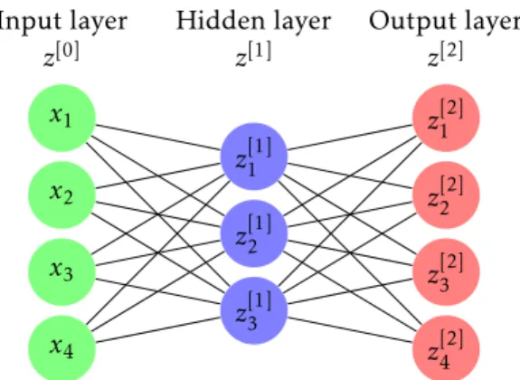
The term feed-in refers to the fact that inputs to a layer depend only on past layers (and not on future layers). Fully connected' refers to the fact that the value of (z[k])j is (possibly) affected by each value of the previous layers, as can be seen from Equation (5.7) and Figure 5.1. Forward neural networks are often used with many layers to construct highly non-linear functions and are often difficult to interpret due to the composite output (Skip-Gram is somewhat of an exception, see Section 5.5).

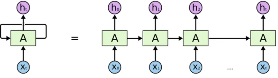
A recurrent neural network (RNN) is a neural network architecture primarily used for modeling sequential data inputs (as opposed to feedforward neural networks, which are not suitable for this).

Loss function, gradient descent and back-propagation

Thus to reduce the notational burden, we leave the sum and simply study the derivatives of the map. The structure of feed-forward neural networks allows us to compute each of these Jacobian matrices in a step-by-step procedure called back-propagation, which we elaborate on in the next subsection. The process of "backpropagating" errors (or derivatives) stepwise to the input is called backpropagation (see [22]) and is the general method used to optimize neural networks with multiple layers.

In this section, we describe backpropagation as a stepwise process for updating the weights in a feedforward neural network.

Skip-Gram

This is done to avoid overestimating (and thus oversampling) of pairs at the beginning of the sequence. It is common practice to update the weights after each (or batch) of samples rather than the total cost function as above. Letz= (wi)j denotes the jth entry in the th column of W (also commonly known as Wji), and consider the derivative of the following picture from equation (5.11).

Therefore, to get a good result, it is important to study each of them and how they affect both the cost function and the interpretation of the model.

Stochastic Neighborhood Embeddings

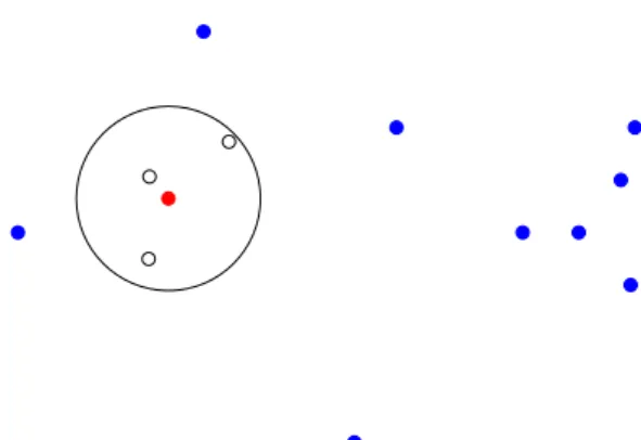
Hereσi2 is a parameter that acts as the variance of the Gaussian distribution and it will be specified later. The heuristic interpretation of this is that for very smallσ, the probability mass is (almost) concentrated in a single point - the nearest point, provided the data points are different. Finally, for SNO this implies that confusion can be interpreted as an estimate of the effective number of neighbors.

For symmetric SNE (with arrow as equation (5.37)) the gradient of the cost function is found to be .

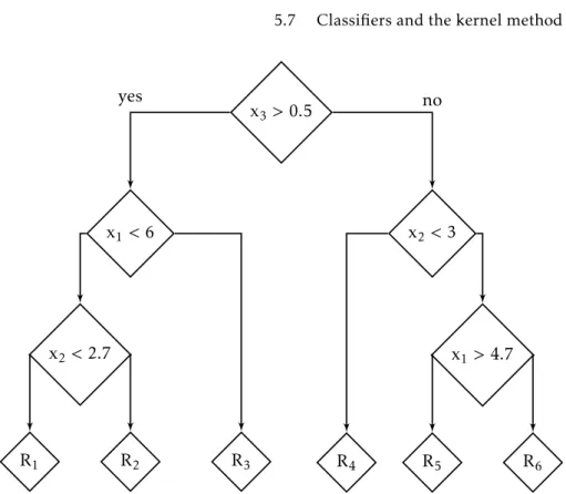
Classifiers and the kernel method

The goal is simply to emphasize that this calculation is not feasible. . the splitting procedure yet). After the completion of the full tree, it is common to "prune" the resulting tree, ie. the lower limit of the Rand index is 0 and the upper limit is 1 – the former indicating zero overlap between two partitions and the latter indicating perfect overlap.

9] Trevor Hastie, Robert Tibshirani and Jerome Friedman. The elements of statistical learning: data mining, inference and prediction.

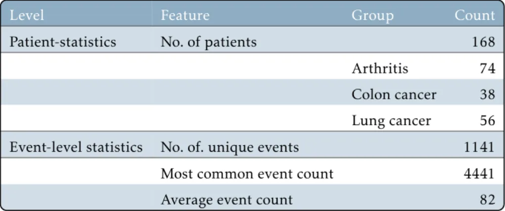
Dataset description

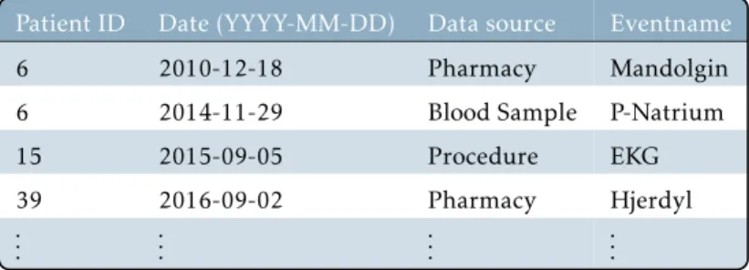
Each sequencej is an ordered set, consisting of items (i.e., entry name or symbol) and is denoted by sj=. for somej∈Nandij∈ I, whereI denotes the set of all unique items in the database Sgiven by. The definition of I allows us to associate each symbol with a unique numeric symbol ID in the natural numbers. In the context of Section 6.2.1, the collection of series corresponds to the data sets of 169 electronic health records (series), which consist of events (items) arranged according to their time and date.

How exactly we use the sequential structure in Section 6.2.2 is a model question, one possible choice is the Word2vec embedding, [16].

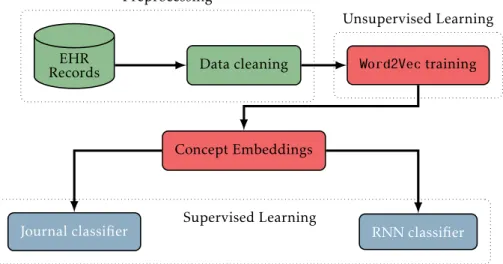
Methods

Continuous Skip-Gram was presented in [16] as an unsupervised learning method for obtaining semantically relevant word representations in natural language processing, with additional computational methods in [18]. The goal of the Skip-Gram algorithm is to estimate the weight matrix W and W0 in equation (6.1). A Skip-Gram data flow graph with input x can be written as a composition of the following mappings.

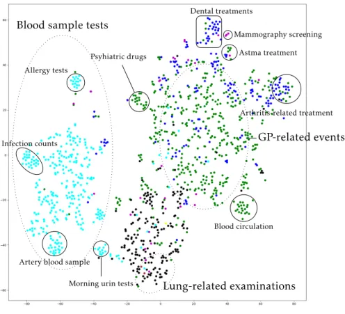
50 Figure 6.2: t-SNE visualization of Skip-Gram event representation with coloring based on data source variable.

Results

The classification algorithms were implemented using the default algorithm configuration in the scientific computing library [23] for Python. Accuracy is measured as the percentage of cluster within the same unsupervised cluster from k-means. We observe that k-means successfully groups several labeled groups into the same clusters.

In the first method, the prediction of the next event is an event in the immediate vicinity of the average contextual representation of the event, e.g.

Conclusion

In the first data set, we study the medication order for patients for whom an alert for sepsis is registered when they are admitted. This data set is divided into two groups during a trial period – in one group an alert is simply registered and in the other group it is registered and sent to a doctor pager. It is not confirmed in the data set whether the patients actually had sepsis or not.

In the second, much larger, dataset, we also study the medication order and the graph of treatment packages (introduced in the next section).

Data collection and datasets

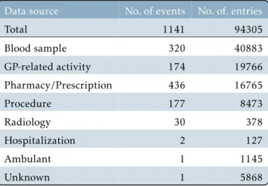
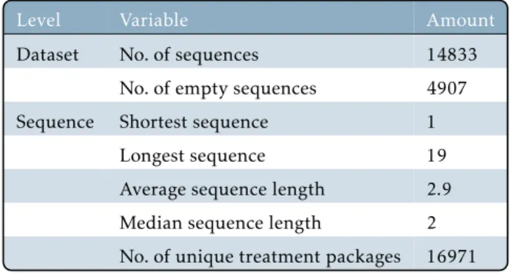
Unfortunately, timestamps are noisy and inaccurate - this is part of the data collection pipeline, as we use the timestamp at which the data is entered (other timestamp choices are not always available). The characteristics of the first data set are described for both groups in Table 7.2 and Table 7.3. The pooled dataset consists of the two datasets and they were crossed on duplicate patients and sepsis records.

The goal of the analysis of the pooled dataset is to visualize the graph to search for rare subgraphs and to predict the next medication using a Markov Chain.

Methods

From the average length of the sequence it is clear that we cannot expect a deep analysis when we often only have 2 or 3 drugs during the 24 hour time period. This leads to a large MC state space since a given set of items may contain all the unique elements I. Note that we have removed the empty sequences from the data set, but mention them since they are a essential part of the original data set.

Due to the average length of the sequences, it is only possible to use a first-order Markov chain.

Results

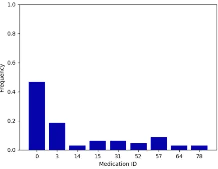
Finally, in section 7.4.3, we test whether a Markov Chain can be used to predict the next medication. In this section we analyze the differences in the treatment packages between the two groups of the first dataset. These graphs show that the frequent medications for both groups are very similar and the only moderate difference is the cumulative frequency of the remaining states.

We included a NO-MED token in each hour slot of the 24-h time window after an alert to investigate whether the number of NO-MED tokens could be a feature separating the control and active group.

Conclusion and perspectives