Phd thesis

(1)

Heavy-Tailed Lévy-Driven Moving Averages

Estimation and Limit Theorems

Mathias Mørck Ljungdahl

Department of Mathematics Aarhus University

2020

(2)

PhD thesis by

Mathias Mørck Ljungdahl 201205667

Department of Mathematics, Aarhus University Ny Munkegade 118, 8000 Aarhus C, Denmark Supervised by

Professor Mark Podolskij

Submitted to Graduate School of Natural Sciences, Aarhus, 31 August 2020

M M L

Monograph was typesat in British English under the Oxford style using kpfonts with

pdfLATEX and the memoir class DEPARTMENT OF MATHEMATICS

AARHUS UNIVERSITY

AU

(3)

Preface

The thesis in hand is the result of my PhD studies from 1 September 2017 to 31 August 2020 under supervision of Professor Mark Podolskij at the Department of Mathemat- ics, Aarhus University.

This treatise encompasses the following five papers which can be read independ- ently, but several of these contains natural links to each other.

Paper A A limit theorem for a class of stationary increments Lévy moving average process [sic] with multiple singularities.Modern Stochastics: Theory and Applications5(3), 297–316.

Paper B A minimal contrast estimator for the linear fractional stable motion.Statis- tical Inference for Stochastic Processes23, 381–413.

Paper C A note on parametric estimation of Lévy moving average processes.Springer Proceedings in Mathematics & Statistics294, 41–56.

Paper D Multi-dimensional normal approximation of heavy-tailed moving averages.

Submitted.

Paper E Multi-dimensional parameter estimation of heavy-tailed moving averages.

Submitted.

Besides minor corrections in terms of spelling and typographical adjustment, the Papers A–E agree with the submitted or accepted versions. While Paper A was tech- nically finished during my part A studies it was not included in the progress report due to page constraints. Moreover, parts of the necessary arguments was included in my master thesis. Paper B was partially included in the aforementioned progress report but critical additions and corrections has been made before its completion and subsequent submission and acceptance. In extension of Paper B I would like to thank Dmitry Otryakhin for collaboration culminating in the inclusion of the estimation techniques from this paper into the R-package rlfsm^(∗). Paper C was included in the aforementioned report almost as is. Papers D and E have been developed and completed in part B of my PhD studies.

The dissertation starts with an introductory part which partly serves to motivate the use of Lévy-driven moving averages and more specifically the heavy-tailed setup.

Secondly, this part also raises classical and always relevant statistical question, and relates the questions to previous literature. Thirdly, a summary of each paper is given relating them not only to the previously mentioned questions, but also internally.

Indeed, Papers B–E have a natural line of thought and development which hopefully will be come clear.

The three years of studies culminating in this treatise is at its end and my gratitude for the resulting journey cannot be expressed in a few words, but I shall try anyway.

(∗) See https://gitlab.com/Dmitry_Otryakhin/Tools-for-parameter-estimation-of-the-linear-fraction al-stable-motion

(4)

multitude and quality of which was appropriate and suitably for my slightly idiosyn- cratic way of study. I will not try to express my internal reaction the day you offered me a chance at a PhD, you can of course guess it.

I thank moreover Christoph Thäle from Ruhr University and Ehsan Azmoodeh from University of Liverpool for a highly efficient and fun collaboration. In a similar note, Danijel Grahovac deserves my gratitude for not only providing and commenting on data, see Figure 2, but also discussing possible model applications.

A thanks goes out to my colleagues at the Department of Mathematics at Aarhus University, including Andreas Basse-O’Connor for many mathematical discussions and his general interest. Thank you also Vytaute Pilipauskaite for your voluminous laughter and our conference trips together.

I would especially like to mention my officemates Thorbjørn Ø. B. Grønbæk for always being cheerful and Mikkel S. Nielsen for fruitful collaboration, discussions and your interminable stream of questions.

I thank of course Lars ‘daleif’ Madsen for providing expert L^ATEX-commentary and specialized solutions.

Noblesse obligecompels me to mention my family and friends; you have shown me that the world is not driven by Lévy processes but by the moments of everyday life—whether or not this is a heavy-tailed distribution I leave uncontested.

Lastly, but certainly not least, an immense gratitude goes to my girlfriend Michelle Lovring—your support and understanding has helped more than you probably know, you have been the Tinúviel to my Beren, the window to my wall.

Mathias Mørck Ljungdahl August, 2020

(5)

Summary

This thesis concerns continuous-time Lévy-driven moving averages with deterministic kernels. These are motivated as a noisy component of a more general model using intuitive concepts and then deduced and specified by more rigorous mathematical theorems. The driver will use a heavy-tailed distribution chiefly to accommodate certain real-world phenomena such as rare events being non-negligible in terms of a probabilistic analysis. The endeavour is to understand the possible dynamics of such driven moving averages—indeed, this is key to extracting or inferring central aspects of the chosen model from actual data. In more concrete terms, using, extending and proving novel limit theory for variational statistics, e.g. the power variation, of given stationary data in this heavy world we shall develop a statistical methodology which allows inference and in particular estimation in a large class of parametrized Lévy-driven moving averages for which the dynamics are allowed to be surprisingly preposterous. Even more concretely, we shall, among other tasks, derive first- and second-order asymptotics for an estimator which finds the optimal parametric model by comparing, under a suitable weighing, the variational statistic of the empirical distribution with the theoretical counterpart of a possible distribution provided by the model—a procedure aptly named theminimal contrast method.

(8)

(9)

Resumé

Denne afhandling omhandler Lévy-drevne glidende gennemsnit i kontinuert tid med deterministiske kerner. Disse gennemsnit vil blive motiveret som en støj-komponent af en mere generel model, ved hjælp af intuitivt klare koncepter og derefter deduceret og specificeret med stringente, matematiske sætninger. Den drivende kraft vil følge en tung-halet fordeling, hovedsageligt for at afstedkomme fænomener fra virkelighedens verden, såsom sjældne hændelser der ikke er negligerbare set fra sandsynlighedsteo- retiske overvejelser. Formålet vil være at forstå de mulige dynamiske egenskaber ved disse sådan drevne glidende gennemsnit – dette er nemlig nøglen til at ekstrahere eller ekstrapolere centrale aspekter af den valgte model fra data. Konkret set vil vi i denne tunge verden bruge, udvide eller bevise ny grænseværditeori for variation- er, som for eksempel kvadratisk variation, af given stationær data til at udvikle en statistisk metodologi som muliggør ekstrapolering og i særdeleshed estimation i en stor klasse af parametriserede Lévy-drevne glidende gennemsnit, hvis dynamiske egenskaber kan tillades at være helt henne i det absurde. I endnu mere konkrete termer, så skal vi, blandt andet, udlede første- og andenordens asymptotik for en estimator som bestemmer den optimale parametriske model ved at sammenligne, under passende vejning, variationen af den empiriske fordeling med den teoretiske pendant stillet tilrådighed af modellen – en procedure som passende kaldesminimal-kontrast metoden.

(10)

(11)

Introduction

This part offers a mostly informal introduction to the class of heavy-tailed Lévy-driven moving averages. We shall in particular deduce this class as a (noise) component of a general time series model. Then the aim of this treatise will be formulated and a very rough overall methodology to tackle this will be sketched. This methodology will then in turn be used as a motivation for each individual paper.

Stationarity and Heavy-Tailed Models

Any analysis of a time series entails the study of the underlying dynamics of the system at hand and any proper analysis will identify components which are fairly homogeneous in some regard. Indeed, theclassical decomposition modelof a time series (Xt)t∈T reads as

X_t=T_t+S_t+Y_t, (t∈T), (1)

consisting of a trend (T_t)_t_∈T, a seasonal or periodic component (S_t)_t_∈T and a noise process (Y_t)_t_∈T. Different standard methods exist for either estimating the trend and seasonality components or transforming (Xt) appropriately, such as taking (higher order) increments at possibly different rates, so we are left with the noise term (Yt), see [14, Section 1.4]. A frequent assumption on the noise is some kind of statistical equilibrium, such as a symmetrical variation around a mean both of which are constant in time, or a mean reversion over time. This leads to the class of (weakly) stationary processes as a model for the noise component (Yt) which we shall discuss in the coming text.

Regardless of the type of observations (e.g. high or low frequency) of our data set let us assume a continuous-time setup as such is reality, in short setT=R. Suppose for the time being that we may formulate the aforementioned equilibrium in the classical, rigorous terms of expectationEand (co)variance Cov; then homogeneity in time of these quantities could be defined as

E[Yt]≡m∈R and Cov(Yt+h, Y_h) = Cov(Yt, Y₀) for allh, t∈R, (2) allowing the covariance to be time-dependent but not the individual variance. Prop- erty (2) is known in the literature as weak stationarity or sometimes as second-order stationarity. Let us glance over the seemingly innocuous implication that (Y_t) now belongs to L²(P) and hence the powerful tools of harmonic analysis and Hilbert space theory are at one’s disposal. Under fairly mild regularity conditions on the auto- covariance function in (2) thenY_t, if centred, will admit a Wold-type decomposition (see [54, 29]):

Y_t= Zt

−∞g(t−s)dL_s+ξ_t (3)

consisting of a casual moving average and a termξ_twhich is essentially known in terms of the observationsY_tfrom the beginning of timet=−∞; see the formulation

(12)

in [2, Theorem 4.1]. Here (Ls) is a square integrable process with weakly stationary and orthogonal increments, and the integral should be understood as anL²-limit of simple functions. The kernelgis a square integrable Borel-measurable function, also known as the spectral density. Assuming additionally that the auto-covariance at (2) is an absolutely continuous function with respect to the Lebesgue measure the term (ξ_t) vanishes and (Y_t) reduces to a casual moving average.

While (3) provides a moving average structure for a large class of noisy components it necessarily does not provide much information besides the second-order properties of (Yt) and additionally, for modelling certain dynamics of the given system, it would therefore be desirable to put extra properties on (L_t), see the introduction in [38]. Alluding instead to the discrete-time setup (such as MA(∞)-processes, see [14]) a natural noise component (Yt) would be driven by i.i.d. observations (Lt).

But unfortunately no such, even remotely, nice process can exists, even if we drop the assumption of square integrability. Indeed, if (Lt)t∈Ris any i.i.d. collection of random variables with a bi-measurable version, then at least one variable would be independent of itself and hence this and therefore all of the collection would be degenerate, see [26, 19] for more on this.

Thus quite naturally (3) inspires us to instead consider dynamics as in (3) with drivers having stationary and independent increments. Requiring independent increments instead of orthogonal allows a framework beyond square integrability for our driver. Assuming slightly more than simply bi-measurability a driver must necessarily be a (two-sided) Lévy process, see [51, 1] for an introduction to Lévy processes and infinitely divisible distributions. Now, in this generality the moving average at (3) can no longer be defined inL²-terms, but rest assured we shall return to this problem later. These driving processes are sufficiently flexible to warrant an already extensive and increasing literature on continuous-time Lévy-driven moving averages.

To name simply a few contributions in this area, dependence properties such as the semi-martingale property [6] and path properties [46] has been studied. Mixing conditions [15, 23] exists and uniqueness of the kernel [47] is understood, both of which are crucial in the inference realm of study. The former is crucial in first-order limit theory and the latter in proper parametrization or specification of a moving average model.

It would also be appropriate to name a few common and popular classes of Lévy- driven moving averages. The first example is the Ornstein–Uhlenbeck process with kernelg(s) = e⁻^λsand for a non-Gaussian driver the authors of [5] show that certain stylized facts from finance can be modelled by this class. One example generalizing the Ornstein–Uhlenbeck is the CARMA processes, whose kernel may be represented as sum of exponential terms, see [13]. Another example generalizing the Ornstein–

Uhlenbeck process are the so-called stochastic delay differential equations, see, e.g.

[9]. The common trait of these models are that they are defined through equations which govern their dynamics directly rather than specify the kernelgexplicitly, which is obviously enticing from a modelling viewpoint.

On the other hand, certain kernel behaviours are known to be, at least on an intuitive level, reflected in the moving average process. For example a non-smooth behaviour at 0 leads to more erratic local behaviour and a slowly decaying tail ofg results in longer memory of the process. This leads more or less directly to the class of fractional Lévy processes that has power law kernels. Foreshadowing, we shall also

(13)

Stationarity and Heavy-Tailed Models

In systems where the underlying dynamics are propelled by gradual smaller changes, the assumption of light tails or even as little as square integrability is definitely satisfied. It is disastrous, even catastrophic, if light-tail modelling is applied to systems where the governing, sovereign unit is large movements. Indeed, in the heavy-tailed spectrum and in general the field of extreme-value theory rare events have a non- negligible probability and it would be ruinous to ignore such events. For example, value-at-risk estimation would be so stupendously offthat it would be useless. These systems arise many places such as, but not exclusive to,

• Insurance claims, see Figure 1.

• Financial data, e.g. stock market returns, see for example [45, Section 1.3.2].

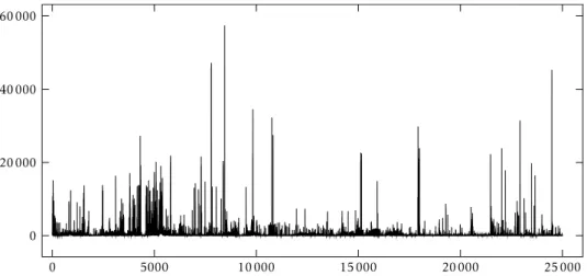
• Data networks, such as LAN packet traces. See also Figure 2.

1980 1981 1982 1983 1984 1985 1986 1987 1988 1989 1990 1991 50

150 250

Figure 1.Fire loss insurance claims in units of 1 million DKK from the period of 1980 to 1990, adjusted for inflation.

Moreover, many common distributions have a fat tail, such as the log-normal and t-distribution, just to mention a one-sided and a two-sided example.

Judging whether or not the data is heavy-tailed or not and how heavy is obviously crucial, but let us remark that some standard methods of assessment exist, see again [45] and let us suppose from now on that this assessment has been answered in the affirmative. Of course in the heavy-tailed setup we do not necessarily have any Wold decomposition to motivate the choice of a moving average structure for the noisy component. Even more grievously, does any quantity resembling a convolutional structure between the Lévy process and the kernel exists? In layman’s terms, we need to properly define Lévy-driven moving averages. Luckily, not only sufficient but also necessary conditions in terms of the characteristic triplet forL, as provided by the Lévy–Khintchine formula, are given in [44] which specify the class of deterministic kernelsgfor which the integral can be defined as a limit of simple functions—see also [23] for the multivariate matrix-valued case. For modelling or simply general interest, it is worth remarking that the theory of Lévy-driven moving averages can be extended to predictable,randomkernels, see [30], or [25] for a brief summary of basics.

(14)

0 5000 10000 15000 20000 25000 0

20000 40000 60000

Figure 2.Ethernet trace recorded at the Bellcore Morristown Research and Engineering facility (BC-Oct89Ext). Packet arrival times in seconds against number of packets in bytes. The data has been aggregated to arrival times in blocks of 1 s and only the 25000 first points are included.

Unfortunately our previous definition of statistical equilibrium through the covariance or expected value is no longer viable—consider, e.g. the extreme, but classical, Pareto distribution with tail index<1. And therefore the definition ofweakstationar- ity is not meaningful, and instead we must rely on the stronger requirement (when both concepts are meaningful) of stationarity, meaning that the finite dimensional distributions

(Y_t₁+h, . . . , Y_t_n+h), (t1, . . . , t_n∈R),

are invariant under the shiftsh∈R. If we still assume symmetry of our noise, then one natural candidate would be the class of symmetricα-stable (SαS) distributions. These are natural partly since they are infinitely divisible and closed under convolution and scaling, but maybe chiefly since they are the universal (central) limits of (sym- metrically distributed) sums of i.i.d. random variables—withα= 2 corresponding to the normal distribution and the classic central limit theorem.

This discussion puts our noise in the class of stationary SαS processes and while we no longer have a Wold-type decomposition, [48, Theorem 6.1] argues that

Y_t=X_t¹+X_t²+X_t³ (4)

with equality in distribution. Here (X_t¹) is a so-called mixed moving average, which can be thought of as superposition of moving averages, (X_t²) is a harmonizable process (see [50]) and (X_t³) is a stationary SαS process which is neither a moving average or harmonizable process, but is, as of now, unsatisfactorily described. Since the components in (4) are mutually independent a study ofY_tcould be split into an analysis of each component separately. As a side-note (4) shows that for SαS processes stationarity and harmonizability are not the same, which is in stark contrast to the Gaussian case, where almost all Gaussian processes have both a harmonizable and a moving average representation, see [22]. This speaks volumes of the flexibility of stationary SαS processes, at least compared to stationary Gaussian processes. But as might be apparent from the discussion so far, we will focus solely on the (non-mixed) moving average part in this dissertation.

(15)

Inference, Simulation and Limit Theory

Lastly, let us remark that there is nothing wrong with a Gaussian driver as our Lévy process. Indeed, quite interesting phenomenon such as turbulence, [20], could be modelled with such processes. The limit theory is quite developed for a Brownian process, even for random volatility kernel functions, known as Brownian semi-stationary processes, see [3, 24]. We will therefore focus on the processes without a Gaussian part and their corresponding novel and emerging limit theory.

Inference, Simulation and Limit Theory

Now that we have settled on the class of SαS moving averages as a potential model forY the ensuing quest becomes manifold. It includes in particular the inference of the kernel functiongand Lévy-driver. In the following we will discuss the overall elements in our study.

To better encompass the processes studied in the treatise we first generalize the SαS moving average processes and considerstationary increments Lévy-driven moving averagesY= (Yt) given by:

Y_t= Zt

−∞(g(t−s)−g₀(−s))dLs, (t≥0), (5) whereg, g0:R→Rare deterministic Borel-measurable functions both of which vanishes on (−∞,0). Moreover,L= (Lt) is a symmetric Lévy process withL₀= 0 with no Gaussian part. The extra functiong₀compared to the moving average in, e.g. (3) does more than simply make the moving average ‘two-sided’. Indeed, data (X_t) accord- ing to the general decomposition model at (1) may very well be transformed using, e.g. increments, which in turn will transform theY at (5) into a proper (stationary) moving average. In other words, (5) allows for a ‘noise’ component which only after transformation of the data is stationary. Moreover, the caseg₀=gis necessary for fractional processes and taking ag0different fromgwould be akin to the inclusion of some initial term.

The point of departure for inference in any (sufficiently complicated) model is in the frequentist world often asymptotic theory. This includes first-order limit theory, often associated with the ‘law of large number’. Indeed, this first order describes what the quantity at hand fluctuatesaround—the common example being the mean.

This is often enough for estimation of a particular characteristic of the underlying model, but we have not describedhowour quantity fluctuates. The ‘central limit theorem’ is used to describe how the empirical average fluctuates around it’s ‘true’

value—in the classical case the description is via weak convergence to the normal distribution at some rate, often√

n. If this second-order limit theory is obtained it allows the construction of asymptotic confidence regions paving the way for a more refined inference.

We describe now the quantities of interest in our particular setup, which are of the type:

V_n(Y;f) =1 n

Xn i=1

f(∆_iY), (n∈N), (6)

wheref :R→Rbelongs to a suitably large class of functions and∆_iY =Y_i−Y_i₋1

denotes the increment. Note that the ergodic theorem dictates thatV_n(Y;f) fluctuates around the meanE[f(∆₁Y)] if the latter is finite.

(16)

A classical example off includes the power variation and it is incessantly studied in the setting of (Itô) semi-martingales, see for example [28, 4, 43]. Providing first- and second-order limit theory in this setting gives a direct inference-link to the integrated volatility of a financial model—a crucial and fundamental quantity.

For certainf we may in general extract important information of the underlying model of (Y_t) via the quantityE[f(∆1Y)], such as in the case of quadratic power variation. To be more concrete, suppose a parametric model{P_θ|θ∈Θ}for (Y_t). Then it might be possible to extract any valueθ fromE_θ[f(∆1Y)] using a particularf. Since only the empirical version,V_n(Y;f), is available from our data it would be natural to consider a comparison map:

θ7−→ρV_n(Y;f),E_θ[f(∆1Y)], (7) for some ‘distance’ρ. Asymptotically it holdsV_n(Y;f)≈E_θ

0[f(∆₁Y)] for the true parameterθ0, so the argument that minimises the distanceρ should be close to θ₀—under suitable injectivity assumptions of course. This idea lies at the heart of the minimal contrast approach. Settingf_u(x) = e^iux, (7) then compares the empirical characteristic function with the theoretical one as a function of the model parameters.

In other words,ρcompares the empirical distribution with theoretical distribution P_θ.

Consideringfu for only a fixed valueu∈Rseems arbitrary and instead we shall consider a minimal contrast estimatorθ_nby comparing all function values:

θ_n= argmin

θ∈Θ

Z_∞

0

V_n(Y;f_u)−E_θ[f_u(∆1Y)]

2µ(du)Cargmin

θ∈Θ

F(Y_n, θ), (8) whereµis a (symmetric) probability measure onRwhich weighs the contrast suitably.

θ_nis an M-type estimator and by differentiation it is turned into aZ-estimator, that is,θ_nis determined by solving theestimating equation:

∇θF(Y_n, θ) = 0.

General theory exists for M- and Z-estimators, see [53], and knowing this it should be apparent that limit theorems for quantities of the typeV_nat (6) are crucial. Indeed, if we are to have any success, then the quantities thatθ_n minimizes over should themselves converge. We remark that with these observations that a possible approach would be to deploy the machinery of empirical process theory as is often done for M- and Z-estimator, but the classical theory requires at least independence and for, e.g.

stationary processes this field is still an active field of research. Instead we shall make use of the implicit function theorem for infinite dimensional spaces; a technique which does have some similarity with the so-calledlinearizationargument, see again [53] or [27]. But instead of trying to fit a square peg into a round hole we formulate the methodology without mention of this type of argument, see, e.g. Section 4.2 in Paper C.

Lastly, for various inference procedures such as parametric bootstrap methods it is of fundamental import to be able to resample from the modelP_θ. As of now, no exact procedure for simulating directly from (5) exists, but for specific subclasses it may

(17)

Paper A

be possible to find quite suitable methods. The general simulation method in the coming text comes as no surprise. Consider in the following an ordinary moving averageY at (5) withg0≡0. For a fixedt∈Ntruncate first the integration region to [−M, t] and then approximate the integral with a Riemann sum of mesh size _m¹, m∈N. Consider then a fixed element of the Riemann sum and write it as a trivial integral with respect toL. This can then be paired with a corresponding term in the truncated integral yielding an error term of the form:

Z _k

k−1(g(t−s/m)−g(t−k/m))dL_s/m, (k∈ {−mM+ 1, . . . , mt}).

IfLis anα-stable Lévy motion, then this is anα-stably distributed error term. Since anyL^p-moment,p < α, of anα-stable random variable can be expressed as a constant times its scale parameter, see [50, Property 1.2.17], it is sufficient to provide bounds on the scale parameter. It is now clear that the error analysis boils down to two behaviours of the kernel: the one at 0 corresponding to the error from the Riemann sum approximation, and the tail decay corresponding to the truncation of the integral.

For bounds in terms of concrete behaviours see [39] and note in particular a potential trade-offbetween the truncation parameterM and the mesh sizem. For a whole sequenceY1, . . . , Y_n one would then need an efficient way of computing the many Riemann sums. This is possible using a Fast Fourier Transform algorithm based on a convolution form of the Riemann approximation—see [52] for the specific example of the linear fractional stable motion. We conclude that parametric bootstrap procedures are often possible in the general setup, see also Paper B.

Paper A

In Paper A we derive a first-order limit theorem for the power variationf(x) =|x|^p at (6) for high frequency observations from thekth order increments ofY:

∆ⁿ_i,kY= Xk j=0

(−1)^j^k j

Y(i−j)/n, i≥k. (9)

Before proceeding with the specific investigation of the current paper we note that limit theorems of (9) for power variations have been investigated in [8] and later generalised in [7] to a larger class of functions which in particular includes bounded functions, such as the (real part) of the characteristic functionf_udiscussed in the previous section. In parallel, a generalisation for the power variation to semi-stationary case is given in [12], which constitutes a class with kernels modulated by a random volatility term.

The aforementioned limit theory shows that not only does the mode of convergence (weak or in probability) but also the type of limit (deterministic or random) depend in a non-trivial way on the interplay between the order of increments,k, the Blumenthal–Getoor indexβ∈[0,2] ofL(see equation (1.4) in Paper A), the behaviour of the functionalgat 0 and the type of functional at hand, where the later type in the power variation case references the specific powerp >0. The behaviour ofg at the point 0 is defined in terms of a power law equivalence in the sense that

g(t)∼t^α ast↓0 (10)

(18)

forα ∈R, where the equivalence f(t)∼g(t) as t ↓0 means that f(t)/g(t)→1 as t↓0. [8] then provides (under some additional conditions, see Assumption (A) and Assumption (A-log) in Paper A) three possible regimes for the ‘law of large numbers’

of the power variation:

(i) Ifα < k−1/pandp > βthenV_n(Y;p) convergesweaklyto arandomlimit at rate n^αp.

(ii) Ifα < k−1/pandp < βthenV_n(Y;p) convergesin probabilityto adeterministic limit at raten⁻^1+p(α+1/β).

(iii) Ifp≥1 andα > k−1/(β∨p) thenV_n(Y;p) convergesin probabilityto arandom limit at raten⁻^1+pk.

Note that in the regime (i) 0 is a singularity ofgin the sense that thekth derivative g^(k)explodes at 0 due to the behaviour (10). This regime is also strikingly different from the case of semi-martingales withp-summable jumps, see, e.g. [28]. The main purpose of Paper A is to investigate the situation of multiple singularity points 0 =θ0<···< θl:

g(t)∼ |t−θ_z|^α^z ast→θ_z (z= 1, . . . , l).

We remark that a similar question is carried out in [24] in the case of Brownian semi-stationary processes. Paper A shows that each singularityθ_zpropagates through to the limit variable in a similar manner to the point 0, except that the propagation depends directly on the fractional size of the resulting blow-up of the singularityθ_z. Indeed, we extend the result from (i) to multiple singularities for any subsequence (n_j)_n_∈N⊆Nsuch that the fractional limit

jlim→∞{njθ_z}Cη_z for eachz∈ {0,1. . . , l} (11) exists. Hence the generalisation of (i) to multiple singularities is even more peculiar than the ordinary case since different subsequence (nj) can lead to differentη_z’s at (11), so the power variation (Vn(Y;p))n∈Nis in general only tight and with multiple accumulation points.

We note that (i) has as a critical case:α=k−1/p. This case has been dealt with separately in article [10] and Paper A also studies this particular case, which for multiple singularity points corresponds toα1=···=α_l=k−1/p.

Before concluding it is worth noting that [8] also provides second-order limit theory which in particular displays the multitude of possible limits: central, non- central, Gaussian and non-Gaussian cases.

Paper B

This article studies thelinear fractional stable motion(lfsm) which corresponds to Y at (5) with the polynomial type kernel:g(s) =g₀(s) =s^H₊⁻^1/αwheres₊= max{s,0}, H∈(0,1) andLis symmetricα-stable Lévy motion with scale parameterσ >0. As we shall now discover, the lfsm can be motivated in several ways. First, the integral at (5) in this case is a direct analogue to the moving average representation of thefractional Brownian motion(fBM)B:

B = Zt

(t−s)^H⁻^1/²−(−s)^H⁻^1/2dW, (t≥0),

(19)

Paper B

whereW= (Wt) is a zero-mean two-sided Brownian motion, cf. [36]. The lfsm is in this regard a generalisation which contains the fractional Brownian motion as the special case:α= 2. The wide applicability of the fBM can then be transferred to the lfsm and actually much empirical data exhibits theJosepheffect, commonly known as long range dependence of increments—a trait the fBM is famous for. Additionally, data may also display what is known as theNoaheffect, which in a nut shell is larger governing dynamics. This latter effect is not displayed by the light-tailed distribution of the Gaussian process, but it is by the SαS-distributed marginal distributions of the lfsm. Moreover, initially, for simplicity and lack of probabilistic tools, the two effects where modelled separately, see [35] for more information. The lfsm may therefore capture both effects. Of course, long range dependence is not understood in the classical sense of a slow decay of the auto-correlations but instead of a slow decay of the (incremented) kernel:

x^H⁻^1/α−(x−1)^H⁻^1/α∼Cx^H⁻¹⁻^1/α asx→ ∞

for some constantC∈R. In a similar note the lfsm can be motivated using fractional calculus, cf., e.g. [42], since these tools are sometimes used to obtain long memory or dependence from a given process—in the lfsm case a SαS Lévy process. Such a procedure has been done in [21] for the aforementioned stochastic delay differential equations to obtain a semi-martingale, contrary to the lfsm, with long-range dependence.

So secondly, the lfsm is also motivated by real-world phenomena. Indeed, the lfsm is considered as a possible model for heavy network traffic, such as Figure 2, since this kind of data is considered to exhibit both self-similarity and heavy tails, see [34].

The fBm is self-similar with (Hurst) indexH∈(0,1), meaning that in distribution:

(B_ct)_t_≥₀= (c^HB_t)_t_≥₀,

and it is the only (up to a scaleσ >0) zero-mean Gaussian process with stationary increments with this property. While the lfsm is also self-similar with indexHit is no longer uniquely determined by this property among the SαS distributions, cf. [16].

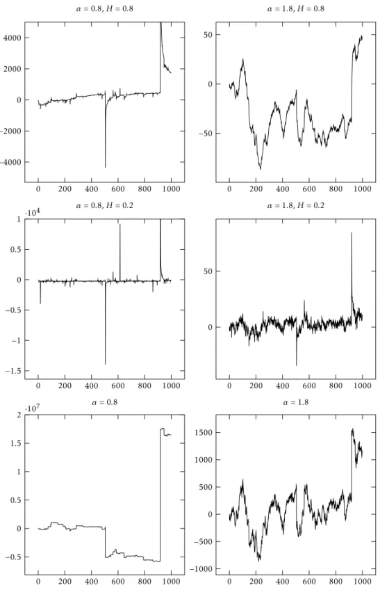
But the contrasting properties of the lfsm and the fBM does not stop here. The path properties of the lfsm are well-known, see [50], but contrary to the fBM which has locally Hölder continuous path of any order< Hthe lfsm has only Hölder continuous paths up to orderH−1/αin the caseH−1/α >0, but if this exponent is negative the lfsm is unbounded on any open interval, see Figure 3.

Parameter estimation of (H, σ) for the fBM has been tackled successfully, see the references in Paper B. But the situation for estimation of the three-dimensional parameter (σ , α, H) for the lfsm has been much more partial in the sense that no estimation of the joint parameter (σ , α, H) together with accompanying second-order theory has been proposed—that is, until recently in [37]. Here the authors proposes a ratio-type estimator for the Hurst parameterHbased on the power variation of thekth orders increments at (9) but at different rates. This is then combined with identities for the characteristic function of thekth order increments to obtain expressions for the scaleσ and stability indexα, see Section 4.1 in Paper B. Moreover, using [8] as a starting point the authors of [37] provide second-order limit theory consisting of a normal regime in the casek > H−1/αand a stable regime whenk < H−1/α.

(20)

0 200 400 600 800 1000

−4000

−2000 0 2000 4000

α= 0.8,H= 0.8

0 200 400 600 800 1000

−50 0 50

α= 1.8,H= 0.8

0 200 400 600 800 1000

−1.5

−1

−0.5 0 0.5

1·10⁴ α= 0.8,H= 0.2

0 200 400 600 800 1000 0

50

α= 1.8,H= 0.2

0 200 400 600 800 1000

−0.5 0 0.5 1 1.5

2·10⁷ α= 0.8

0 200 400 600 800 1000

−1000

−500 0 500 1000 1500

α= 1.8

Figure 3.Top two rows are paths of the linear fractional stable motion and the bottom row is the drivingα-stable Lévy motion.

(21)

Paper B

To obtain the necessary identities for the scale and stability index (σ , α) only two values of the characteristic function are needed, concretely the values att₁= 1 andt2= 2 are used. Hence, as already mentioned, it would be natural to instead compare for all valuest∈Rand therefore consider the minimal contrast estimator θ_n at (8) withθB(σ , α, H)∈ΘB(0,∞)×(0,2)×(0,1). To obtain first- and second- order limit theory we will therefore naturally need limit theorems for the underlying integral functionalFat (8). In Paper B we analyse, extend and develop the necessary arguments for our ‘linearization’ methodology to work. To obtain a weak limit theory for the centred objectn^r(θn−θ) for some rater, three fundamental steps are required:

Step 1 Obtain finite dimensional weak convergence of the underlying processes u7→V_n(Y;f_u)−E_θ[f_u(∆₁Y)].

Step 2 Analysis of the path properties of the limit process obtain at Step 1.

Step 3 Extend the convergence from Step 1 to convergence of the integral functional F(Y_n, θ).

Step 1 has been dealt with in [37] which is necessary for their limit theory, but it is not viewed in the sense of finite dimensional convergence of processes as it is for the minimal contrast estimator in Paper B.

Step 3 is related to the general question of whether finite dimensional convergence of a sequence of processes can be extended to integral functional of these. This has of course been studied before but the available results are not particularly satisfactory for our purpose. Instead we observe that certain moment bounds are sufficient for the extension in Step 3. This is also related to Step 2 since in the normal regime, k > H+ 1/α, we analyse the covariance of the functionals in Step 1 to obtain an expression for the covariance function of the Gaussian limit. This analysis also yields a Hölder continuous version of the limit Gaussian process which concludes Step 2 and here the tractability of the characteristic function of an SαS distributed variable is important since it is directly related to the covariance function of the limit, see Theorem 2.1(i) and the quantity at (2.4) in Paper B.

For the stable regime,k < H+1/α, covariance bounds are not available and instead we prove a Karamata type theorem to provide uniform bounds on the moments of the processes at Step 1, see Proposition 5.7 in Paper B. These moment bounds are not suitable for the analysis of the stable limit process, but this process is extremely simple as it is of the form: (κ(u)S)u≥0, for some deterministic functionκ:R₊→R and some skewedα-stable variableS—making Step 2 a trivial matter in this regime.

After the second-order limit theory has been developed Paper B tackles the question of asymptotic confidence regions for the parameters. The most imme- diate problem is which regime we are in, the normal regime,k > H+ 1/α, or the stable regime,k < H+ 1/α. This is quite crucial since the rate in the stable regime is r= 1−1/(1 +α(k−H)) while in the normal case it isr= 1/2. Since the parameters are unknown the regime and rate is a priori unknown. Moreover, 1/αis unbounded in α∈(0,2) so we cannot simply pick a large incrementk∈N. However, if we are in the continuous caseH−1/α >0, then trivial algebra says that anyk≥2 will place us in the normal regime. In this case Paper B uses a parametric bootstrap approach to build asymptotic confidence regions, see Section 4.2.

(22)

In the general case pre-estimation ofαwill provide an estimate of the necessary orderk∈Nsuch that we may obtain a known rate of√

n-convergence. Unfortunately this yields four different regimes and the limiting type of distribution is no longer known. To overcome this Paper B then proposes in Section 4.3 a subsampling procedure to estimate the distribution functions of the limiting distribution and hence estimate the necessary quantiles for building the asymptotic confidence regions.

We conclude with an unfortunate problem for our general minimal contrast approach. The parameters (σ , α, H) are not completely determined from the (one- dimensional) characteristic function. This forces us to use a plug-in approach by inserting the same ratio estimator as in [37] for the Hurst parameterHin our minimal contrast estimator for (σ , α). In particular we really do need the more complicated limit theory of the variationV_n(Y;f) for unbounded functionalsf.

Paper C

In Paper C we take a step back from Paper B and realize that much of the overall approach, namely Steps 1–3 are generally applicable. Paper C then provides first- and second-order limit theory for the minimal contrast estimator for the class of parametric SαS-driven moving averages, that is, (Y_t) at (5) withg₀≡0 andg=g_θfor a one-dimensional parameterθ∈Θ⊆R. Of course the underlying limit theory at Step 1 from Paper B is no longer available, but theory for generalboundedfunctionals such as the characteristic function has luckily been developed in [41]. For later emphasis we remark here that the functionals inVn(Y;f) are of the type:

f :R−→R^d. (12)

I.e. the co-domain is multi-dimensional, and this is important as it will ensure finite dimensional convergence of our processes induces by the (empirical) characteristic functions. Ifd= 1 then we would only have weak convergence of a single fixed value of our characteristic functions.

As Papers B and C has taught us it would now be foolish to hope that the we can tackle a multi-parametric frameworkΘ⊆R^m with the current methodology. The desire to envelop this framework leads us to the following two papers. The first paper, Paper D, relates directly to Step 1 above and the second, Paper E, completes the second-order limit theory in Steps 2 and 3 for the general multi-parametric framework.

Paper D

The main purpose of this paper is to generalise the limit theory for bounded functionals as in (12) of heavy-tailed Lévy-driven moving averages to multivariate functionals of the type:

f :R^m−→R^d. (13)

This was at the time an interesting question in itself and deserved a specific study, hence the separate, independent article. Our statistical motivation will become clear in the description of the next article, but already now it is intuitively clear that functionals form >1 can capture significantly more complicated behaviour, especially

(23)

Paper D

A very successful method in deriving Gaussian limit theorems has been the combination of Stein’s method with Malliavin calculus. We will sketch the overall (univariate) approach in the following.

Consider a metricd on the space of Borel probability measures onR which metricizes weak convergence. For concreteness consider the Wasserstein distance defined as:

d(Y , N)B sup

h∈Lip₁(R)

E[h(Y)]−E[h(N)],

whereY andNare random variables onRand Lip₁(R) denotes the space of Lipschitz functionsh:R→Rwith Lipschitz constant 1. Recall now Stein’s Lemma which states thatN has a standard normal distribution if and only if

E[f⁰(N)−N f(N)] = 0 (14)

for allf :R→Rin a class of sufficiently smooth functions. So ifY is supposed to be close toN in distribution then replacingN in (14) withY should result in something small. Similarly, the expectations ofh(Y) andh(N) should be roughly the same, or equivalently, the difference should be zero, for a large class of functionsh:R→R. Comparing the two differences then yields, on average,

f⁰(x)−xf(x)≈h(x)−E[h(N)].

Fixinghand replacing the approximation ‘≈’ with an equality yields a first-order differential equation inf known asStein’s equation for normal approximation. For some classes ofhthe functional solutionf to Stein’s equation is known to satisfy certain regularity conditions—e.g. for Lipschitzhas in the Wasserstein distance the solutionf is a continuous differentiable function with absolutely continuous derivative.

Hence we obtain the following bound:

d(Y , N)≤sup

f∈H|E[f⁰(Y)−Y f(Y)]|,

for a certain class of functionsH; we refer to [18] for more details. We have now reduced the problem to terms depending solely onY. Suppose from now on thatY is a Poisson functional, i.e. a function of a Poisson (point) process (on some abstract space). This includes moving averages driven by a pure jump Lévy process, [49, Proposition 2.10], but is not exclusive to these. In this Poissonian framework the powerful tools of Malliavin calculus (on Poisson spaces) are available to us. We refer the reader to [33, 32] for an excellent introduction into this elegant field of mathematics. Indeed, using key formulas it is possible to obtain so-called second-order Poincaré inequalities, where ‘second-order’ simply refers to the fact that bounds on, e.g. the Wasserstein distance leads to second-order limit theorems, see [17]. Correspondingly, these inequalities may involve the analysis of (second-order) Malliavin derivatives.

Until recently the available second-order Poincaré inequalities in [31] where not suitable for heavy-tailed moving averages since the available bounds diverged in this case. This was rectified in [11] and a refined second-order Poincaré inequality was established by careful distinction between small and large values for certain Malliavin derivatives.

(24)

The method of [11] was also the departure for Paper D where the extension to functionals at (13) for a generalm >1 was possible due to the simple, but not simplistic, method. For the extension to (13) for a generald >1 the classical Wasserstein was no longer suitable. Indeed, if we wish to provide bounds between a multivariate normal distribution and our Poisson functional the situation depends on the covariance matrix of the normal distribution—if we do not put any assumption of invertibility on this matrix, then we need to increase the smoothness of the classH, see [40, Table 1]

for a concrete comparison.

Luckily, for our statistical purposes the exact metric is not so important as long as it implies weak convergence and as a corollary of the refined Poincaré inequality in a multivariate setting,m >1, the article provide bounds for a suitably large class of multi-dimensional moving averages. Let us elaborate slightly more on this, consider anm-dimensional random vector (Y¹, . . . , Y^m) of moving averages with

Y_tⁱ = Zt

−∞g_i(t−s)dLs, (i∈ {1, . . . , m}),

where the kernelg_i:R→Rsatisfy certain power law behaviours at 0 and at∞andL is a common SαS-driver. To draw parallels with previous limit theory suppose that

g_i(t)∼t^κⁱ ast↓0 and g_i(t)∼t⁻^βⁱ ast↑ ∞

forβ₁, . . . , β_m>0 andκ₁, . . . , κ_m∈R. Then if the kernel is not too ‘explosive’ at 0, i.e.

κ_i >−1/α, and the underlying common driverLis not too heavy-tailed combined with the memory being not too long, i.e.αβ_i >2, then we obtain a joint central limit theorem for

V_n(Y;f) = 1 n

n

X

i=1

f(Y_i¹, . . . , Y_i^m)

for boundedC²-functionsf :R^m→R^dwith bounded derivatives. We conclude by remarking that this fits our intuition, based on previously established theory such as [7], quite well, and that Paper D generalises the framework off :R→Rin [11] to functionals as in (13).

Paper E

We now return to our previous defeat in Papers B and C. Viz, the methodology has so far only been able to tackle moving averagesY as in (5) withg₀≡0 andg =g_θ for a low-dimensional parameterθ∈Θ. To make this more precise, we consider the theoretical characteristic function of the marginalY₁:

φ_θ(u) =E_θ[exp(iuY1)] = exp(−u^αkgθk^αα), (u∈R) (15) wherekg_θk^αα=R

R|g_θ(s)|^αdsdenotes the ordinaryL^α(R)-norm—this specific form for the characteristic function follows sinceY₁is a SαS-distributed, see [50, Chapter 3].

It seems clear that it is unreasonable to deduce high-dimensional parametersθfrom (15), especially parameters retaining to path or dependence properties such as a self- similarity index. This of course relates to a discussion on uniqueness of the spectral representation of (SαS-) moving averages as mentioned previously; see also [47].

(25)

References

A natural step towards a solution would be to instead consider the characteristic function of the joint distribution (Y₁, . . . , Y_m):

ϕ_θ(u1, . . . , u_m) =E_θ

heⁱ^P^m^k=1^u^k^Y^kⁱ= exp

−

Xm k=1

u_kg_θ(·+k)

α α

and it is empirical counterpart:

V_n(Y;f_u) = 1 n−m

n−m

X

s=0

f_u(Y_s+1, . . . , Y_s+m), (u∈R^m), wheref_u(y₁, . . . , y_m) = exp(iPm

k=1u_ky_k). This immediately places us in the framework of m >1 andd = 1 of Paper D. Moreover, as already mentioned we need to vary u∈R^mto obtain finite dimensional convergence of our (empirical) processes (which are now of course called fields) and therefore we require the full generality of our newly developed framework in Paper D:d, m >1.

Paper E then discusses the assumptions on the kernel and (theoretical) characteristic function necessary for the statistical methodology to work. Indeed, these assumptions falls into two categories; one related to the parameter identification from the m-dimensional marginal distributions as we have just discussed, and a category related to our linearization type argument.

Of course Paper E also studies several important examples including Ornstein–

Uhlenbeck type processes and we are finally able to defeat the lfsm and provide a full minimal contrast estimator for this process without relying on a plug-in method. It should be clear from the general formulation that the methodology could in principle handle a very large class of parametric moving average processes and provide Gaus- sian limit theorems in the case where this is a reasonable goal to pursue, i.e. under appropriate behaviour of the kernelg_θat 0 and∞—as we have alluded to at several times.

References

[1] David Applebaum (2009). »Lévy processes and stochastic calculus«. 2nd edition.

Cambridge Studies in Advanced Mathematics 116. Cambridge University Press.

isbn: 978-0-511-80978-1.doi: 10.1017/CBO9780511809781.

[2] Ole E. Barndoff-Nielsen and Andreas Basse-O’Connor (2011). »Quasi Ornstein–

Uhlenbeck processes«.Bernoulli17(3), 916–941.doi: 10.3150/10-BEJ311.

[3] Ole E. Barndorff-Nielsen, José Manuel Corcuera and Mark Podolskij (2013).

»Limit theorems for functionals of higher order differences of Brownian semi-sta- tionary processes«. In: »Prokhorov and contemporary probability theory«. Edited by Albert N. Shiryaev, S. R. S. Varadhan and Ernst L. Presman. Springer Berlin Heidelberg, 69–96.isbn: 978-3-642-33549-5.

[4] Ole E. Barndorff-Nielsen and Neil Shephard (2003). »Realized power variation and stochastic volatility models«.Bernoulli9(2), 243–265.doi: 10.3150/bj/106 8128977.

(26)

[5] Ole E. Barndorff-Nielsen and Niel Shephard (2001). »Non-Gaussian Ornstein–

Uhlenbeck-based models and some of their uses in financial economics«.Journal of the Royal Statistical Society63(2), 167–241.doi: 10.1111/1467-9868.00282.

[6] Andreas Basse and Jan Pedersen (2009). »Lévy driven moving averages and semimartingales«.Stochastic Processes and Their Applications119(9), 2970–

2991.doi: 10.1016/j.spa.2009.03.007.

[7] Andreas Basse-O’Connor, Claudio Heinrich and Mark Podolskij (2019). »On limit theory for functionals of stationary increments Lévy driven moving averages«.

Electronic Journal of Probability24(79), 42 pp.doi: 10.1214/19-EJP336.

[8] Andreas Basse-O’Connor, Raphaël Lachièze-Rey and Mark Podolskij (2017).

»Power variation for a class of stationary increments Lévy driven moving averages«.

The Annals of Probability45(6B), 4477–4528.doi: 10.1214/16-AOP1170.

[9] Andreas Basse-O’Connor, Mikkel Slot Nielsen, Jan Pedersen and Victor Rohde (2020). »Stochastic delay differential equations and related autoregressive mod- els«.Stochastics: An International Journal of Probability and Stochastic Processes92(3), 454–477.doi: 10.1080/17442508.2019.1635601.

[10] Andreas Basse-O’Connor and Mark Podolskij (2017). »On critical cases in limit theory for stationary increments Lévy driven moving averages«.Stochastics89(1), 360–383.doi: 10.1080/17442508.2016.1191493.

[11] Andreas Basse-O’Connor, Mark Podolskij and Christoph Thäle (2019). »A Berry–Esseén theorem for partial sums of functionals of heavy-tailed moving aver- ages«. arXiv: 1904.06065.

[12] Andreas Basse-O’Connor, Claudio Heinrich and Mark Podolskij (2018). »On limit theory for Lévy semi-stationary processes«.Bernoulli24(4A), 3117–3146.

doi: 10.3150/17-BEJ956.

[13] Peter J. Brockwell (2004). »Representations of continuous-time ARMA processes«.

Journal of Applied Probability41, 375–382.

[14] Peter J. Brockwell and Richard A. Davis (2006). »Time series: Theory and meth- ods«. 2nd edition. Springer Series in Statistics. Springer.isbn: 978-1-4419-0319- 8.doi: 10.1007/978-1-4419-0320-4.

[15] Stamatis Cambanis, Clyde D. Jr. Hardin and Aleksander Weron (1987). »Er- godic properties of stationary stable processes«.Stochastic Processes and Their Applications24(1), 1–18.doi: 10.1016/0304-4149(87)90024-X.

[16] Stamatis Cambanis and Makoto Maejima (1989). »Two classes of self-similar stable processes with stationary increments«.Stochastic Processes and their Applications32(2), 305–329.issn: 0304-4149.doi: 10.1016/0304-4149(89)900 82-3.

[17] Sourav Chatterjee (2009). »Fluctuations of eigenvalues and second order Poincaré inequalities«.Probability Theory and Related Fields143, 1–40.doi: 10.1007 /s00440-007-0118-6.

(27)

References

[18] Louis H. Y. Chen, Larry Goldstein and Qi-Man Shao (2011). »Normal approx- imation by Stein’s method«. Probability and Its Applications. Springer-Verlag Berlin Heidelberg.isbn: 978-3-642-15006-7.doi: 10.1007/978-3-642-15007-4.

[19] Donald L. Cohn (1972). »Measurable choice of limit points and the existence of sep- arable and measurable processes«.Zeitschrift für Wahrscheinlichkeitstheorie und Verwandte Gebiete22, 161–165.doi: 10.1007/BF00532735.

[20] José Manuel Corcuera, Emil Hedevang, Mikko S. Pakkanen and Mark Podolskij (2013). »Asymptotic theory for Brownian semi-stationary processes with application to turbulence«.Stochastic Processes and Their Applications123(7), 2552–

2574.doi: 10.1016/j.spa.2013.03.011.

[21] Richard A. Davis, Mikkel Slot Nielsen and Victor Rohde (2020). »Stochastic differential equations with a fractionally filtered delay: a semimartingale model for long-range dependent processes«.Bernoulli26(2), 799–827.doi: 10.3150/18- BEJ1086.

[22] Joseph L. Doob (1990). »Stochastic processes«. John Wiley & Sons, Inc.isbn: 0-471-52369-0.

[23] Florian Fuchs and Robert Stelzer (2013). »Mixing conditions for multivariate infinitely divisible processes with an application to mixed moving averages and the supOU stochastic volatility model«.ESAIM: PS17, 455–471.doi: 10.1051/ps/20 11158.

[24] Kerstin Gärtner and Mark Podolskij (2015). »On non-standard limits of Brownian semi-stationary processes«.Stochastic Processes and their Applications125(2), 653–677.doi: 10.1016/j.spa.2014.09.019.

[25] Claudio Heinrich (2017). »Fine scale properties of ambit fields: Limit theory and simulation«. PhD thesis.url: https://data.math.au.dk/publications/phd/2017 /math-phd-2017-ch.pdf.

[26] Jørgen Hoffman-Jørgensen (1973). »Existence of measurable modifications of stochastic processes«.Zeitschrift für Wahrscheinlichkeitstheorie und Ver- wandte Gebiete25, 205–207.doi: 10.1007/BF00535892.

[27] Jørgen Hoffman-Jørgensen (1994). »Probability with a view towards statistics«.

Volume II. Chapman & Hall.isbn: 0-412-05231-8.

[28] Jean Jacod and Philip E. Protter (2012). »Discretization of processes«. Stochastic Modelling and Applied Probability 67. Springer-Verlag Berlin Heidelberg.isbn: 978-3-642-24126-0.doi: 10.1007/978-3-642-24127-7.

[29] Kari Karhunen (1950). »Über die Struktur stationärer zufälliger Funktionen«.

Arkiv för Matematik1(2), 141–160.doi: 10.1007/BF02590624.

[30] Stanislaw Kwapién and Wojbor Woyczyński (1992). »Random series and stochastic integrals: Single and multiple«. Probability and Its Applications. Birkhäuser.

isbn: 978-0-8176-4198-6.