Spatio-temporal modelling - Department of Mathematics

The overview provides an introduction to spatio-temporal modeling of growing objects and presents the main results of the companion articles. The main goal of the modeling is to capture different spatio-temporal interactions in an observed growth pattern and try to relate the proposed model to specific biological entities. Issues related to the patterning and progression of the tumor are important, as is the shape.

Being able to describe the morphology of the border of the tumor provides a useful tool to help classify and determine the malignancy. The boundary of an expanding object is modeled in discrete time, by representing the object at the present time as a transformation of the object in the immediate past. A major advantage of these models is the possibility to control the spatiotemporal correlation structure of the expanding object and thus to characterize the morphology of the boundary of the expanding object.

The main characteristic of the supracellular models is that only the macroscopic level of the observed patterns is modelled. However, it is important to construct models with known correlation between the microscopic and macroscopic levels of the biological growth pattern.

The template approach and the p-order growth model

Extensions

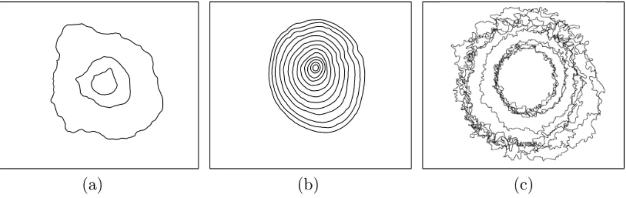
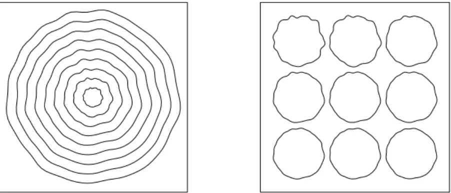
The series{Vt} of stochastic deformation processes are assumed to be independent according to the order growth model. In section 3.1 below, an example of the growth of the year rings of a tree is given. If the number of observed increments is not too small, it is possible to model the dependence on the {Vt} series.

Instead of assuming that the series X = {Xt} is independent and identically distributed, we assume that X = {Xt} is a stationary time series of cyclic Gaussian processes that conform to an ARMA model. Let W = {Wt} be a sequence of independent and identically distributed stationary Gaussian processes on [−π, π), such that Wt∼Gp(0, α, β).

Lévy based models

The induced covariance structure

In this section we will focus on the linear Lévy growth model, but remind you that the results will apply to the logarithm of the vector radio function if it follows the exponential Lévy model. Under these assumptions, it can be shown that the spatial covariances of the vector function Rt are given by. Moreover, if atk =btck, then ρt(φ) does not depend on t and the correlation function R(φ) ={Rt(φ) :t≥0} is determined by the time expansion T(t) of the set of ambients at time t and the function g,.

In a Lévy growth model of the type discussed above, the Fourier coefficients will also follow a linear Lévy growth model. In this section, we will provide examples of the application of the models discussed in Section 2. An analysis of human breast cancer cell islands was presented in Jónsdóttir and Jensen (2005).

The parameters of the second-order growth model µt, αt and βt were estimated and the model fit the data well according to the model control procedures developed by Jónsdóttir and Jensen (2005). In the event that the number of observed increments is large, a more sophisticated hypothesis test can be made, e.g.

Lévy based growth models

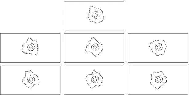
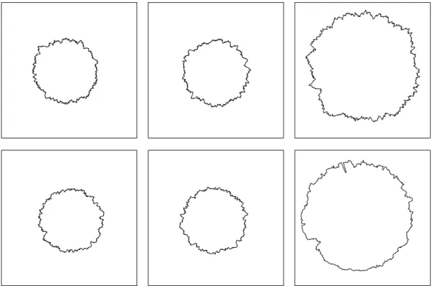
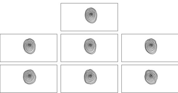
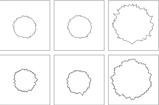
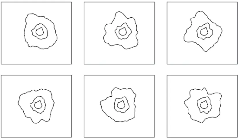
The data set and the simulations in the second and third rows of Figure 3.2 look very similar, indicating that the hypothesis of independent increases is likely to be accepted. It does not seem feasible to describe the growth pattern in Figure 3.1 (c) with a p-type growth model because the profiles are locally very irregular. There are also sudden bursts of profiles that are impossible to model using Gaussian processes with covariance structures based on an ad hoc model.

The data set (top), conditional simulations under the second-order growth model with µt,αt and βt replaced by the maximum likelihood estimates (second row) and simulations under the second-order growth model with independent increments and µt,αtandβreplaced by the maximum likelihood estimates (third row ). The dataset (top), conditional simulations under the second-order growth model with µt, αt and βt replaced by the maximum likelihood estimates (second row) and simulations under the second-order growth model with independent increments and µt, αt and βt replaced by the maximum probability estimates (third row). and the parameters of the model were estimated using mean and covariance estimation for three time points, t. Note that although the overall appearance is similar for the data and the simulation, sudden bursts are present in the data set that are not seen for the simulated profiles.

The parameters of the underlying basis are chosen so that the mean and variance of Rt(φ) are the same as when the Gaussian basis was used. The first row shows a simulation very similar to the Gaussian simulation, but more bursts are observed in the second row.

Circular systematic sampling using the p-order model

As mentioned in Section 2.1, the coefficients λk determine the global fluctuations of F for small k, while for large they determine the local fluctuations of F. Daley and Vere-Jones (2002) treat in detail spatiotemporal point processes defined using this mechanism. 4.2) It can be shown that the density of Zt can be written as. The simplest example of a spatiotemporal point process is the Poisson process with intensity function λ.

A spatiotemporal Cox process on S is simply a spatiotemporal Poisson point process with random intensity function Λ, i.e. As for the spatiotemporal Poisson processes, Xt0 can be obtained from Xt if t0 < t. A large class of spatiotemporal Cox processes can be obtained by modeling the random intensity function by a Lévy-based spatiotemporal model, eq.

Another example, using Lévy-based spatiotemporal models, is a Cox Z process with random intensity. where L is a Gaussian Lévy basis onS, i.e. Note that the intensity function and the pair correlation function of a spatiotemporal Cox process can be easily calculated using the cumulant function ofΛ(ξ, t), i.e.

Extensions of inhomogeneous spatial point processes

There are enormous possibilities to define different Cox processes using this representation. ThenZ is a spatiotemporal shot noise Cox process. As mentioned above, the cumulative spatial processes will also be Cox processes, but not necessarily shot-noise Cox processes. 1998) and Brix and Møller (2001) use a special type of log-Gaussian Cox processes to study weed data.

A simple way to construct a spatiotemporal extension of a pairwise interaction process is to write its density. It can further be shown that ift0 < t, the cumulative point processXt0 can be obtained by independent dilution of Xt. In general, any given point processX in χ can be used to construct a spatio-temporal point process model using backward temporal thinning.

A backward temporal thinning of this type implies that Xt can look like a realization of a Poisson point process for smallt. An alternative procedure for extending inhomogeneous spatial point processes to a spatiotemporal framework is to extend expressions for the Papangelou conditional intensity, used in a purely spatial context, to expressions for the conditional intensity λg(·)f ?(·|·)of the spatiotemporal point process. 2006), this approach and the approach based on backward thinning have been tested in the case where the purely spatial point process is a locally scaled Strauss process, cf.

Dynamic random compact sets

In case the point process Z is Poisson, the model (4.6) is a dynamic version of the well-known Boolean model. The models are discrete time models and the state of the cells at that time is a function of the neighboring cells at the previous time point, where various neighboring relations can be used. The void function F for the arbitrary set Y is given by the distribution function of the distance from the origin to the arbitrary set Y, i.e.

One of the simplest estimators for the empty space function F is based on minus sampling. The distance from a fixed point to the nearest point of the random set is censored by the distance from the observation window. The local version of the survival function is Sξ(r) = 1−Fξ(r) and if the local empty space function is differentiable for allξ ∈Rd and r >0, let fξ be the derivative of Fξ and define the local hazard rate Through.

These kinds of degree of risk transformations occur in the Cox proportional risk model and the accelerated lifespan model, and the two models therefore have the intuitive appeal of describing non-stationary change of intensity and scale, respectively. Typically, the properties of the local empty space function cannot be obtained for known models for non-stationary random closed sets.

Estimation methods

Application to non-stationary point processes

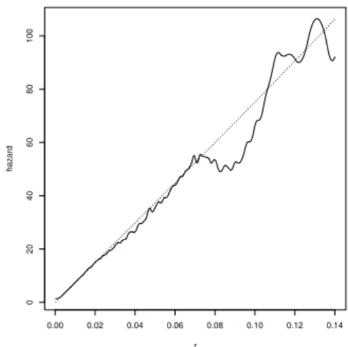
In Section 3, we will define the local version of the empty space function of the nonstationary. It follows that the local hazard rate of a random compact set X at ξ satisfies λξ(r) = exp(β·ξ)λ0(r),. Equations (14) and (16) are used to calculate the local hazard rate of the inhomogeneous Poisson process.

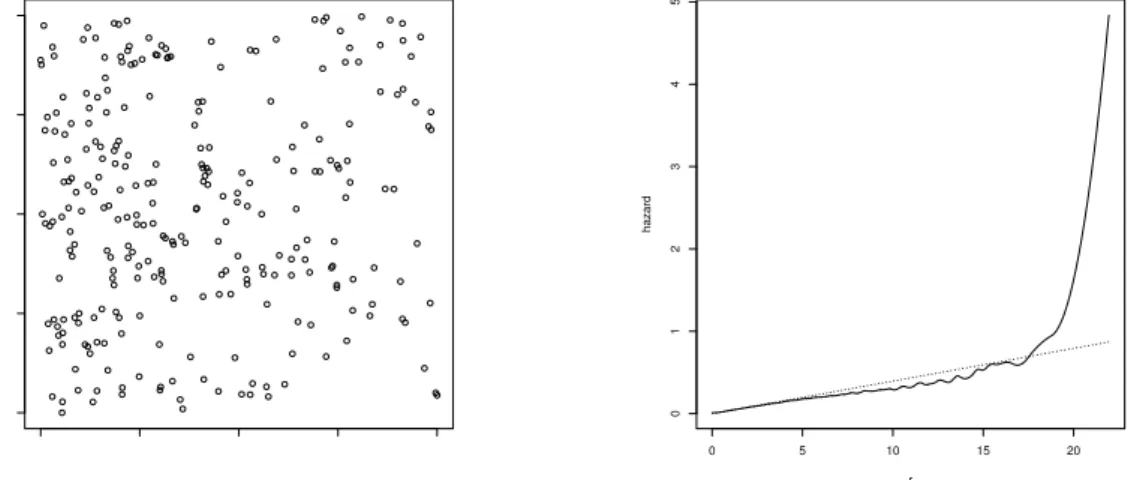
Figure 3 shows the logarithm of the estimated survival function ˆSξ0(r) versus the survival function of the inhomogeneous Poisson process with intensity ˆαexp( ˆβ·ξ).