www.the-cryosphere.net/6/1187/2012/ doi:10.5194/tc-6-1187-2012
© Author(s) 2012. CC Attribution 3.0 License.
The Cryosphere
Sea ice inertial oscillations in the Arctic Basin
F. Gimbert1,3, D. Marsan2, J. Weiss3, N. C. Jourdain4, and B. Barnier4 1ISTerre, Universit´e de Grenoble 1, CNRS, UMR5275, 38041 Grenoble, France 2ISTerre, Universit´e de Savoie, CNRS, 73376 Le Bourget-du-Lac, France 3LGGE, Universit´e de Grenoble 1, CNRS, 38041 Grenoble, France 4LEGI, Universit´e de Grenoble 1, CNRS, 38041 Grenoble, France
Correspondence to: F. Gimbert (florent.gimbert@ujf-grenoble.fr)
Received: 30 April 2012 – Published in The Cryosphere Discuss.: 18 June 2012 Revised: 24 September 2012 – Accepted: 1 October 2012 – Published: 24 October 2012
Abstract. An original method to quantify the amplitude of inertial motion of oceanic and ice drifters, through the in-troduction of a non-dimensional parameterMdefined from a spectral analysis, is presented. A strong seasonal depen-dence of the magnitude of sea ice inertial oscillations is re-vealed, in agreement with the corresponding annual cycles of sea ice extent, concentration, thickness, advection veloc-ity, and deformation rates. The spatial pattern of the magni-tude of the sea ice inertial oscillations over the Arctic Basin is also in agreement with the sea ice thickness and concen-tration patterns. This argues for a strong interaction between the magnitude of inertial motion on one hand, the dissipa-tion of energy through mechanical processes, and the cohe-siveness of the cover on the other hand. Finally, a significant multi-annual evolution towards greater magnitudes of iner-tial oscillations in recent years, in both summer and winter, is reported, thus concomitant with reduced sea ice thickness, concentration and spatial extent.
1 Introduction
The spectacular evolution of the Arctic sea ice cover over the last few decades is not restricted to the shrinking of the ice extent (Comiso et al., 2008; Stroeve et al., 2008), its thin-ning (Rothrock et al., 2008; Kwok and Rothrock, 2009), or, consequently, a continued decline of the ice volume (Lindsay et al., 2009). Kinematics is affected as well, and its evolution plays a central role in the changes currently taking place in the Arctic Ocean. As observed from buoy drift data, the sea ice mean speed over the Arctic increased at a rate of 9 % per decade from 1979 to 2007, whereas the mean
deforma-tion rate increased by more than 50 % per decade over the same period (Rampal et al., 2009). These two aspects of re-cent sea ice evolution, i.e. strong decline in terms of ice ex-tent and thickness, and accelerated kinematics, are strongly coupled within the albedo feedback loop. Increasing defor-mation means increasing fracturing, hence more lead open-ing and a decreasopen-ing albedo (Zhang et al., 2000). As a re-sult, ocean warming, in turn, favours sea ice thinning in sum-mer and delays refreezing in early winter, i.e. strengthens sea ice decline. This thinning should decrease the mechan-ical strength, therefore allowing even more fracturing, hence larger speed and deformation. A consequence is the acceler-ation of the export of sea ice through Fram Strait, with a sig-nificant impact on sea ice mass balance (Rampal et al., 2009, 2011; Haas et al., 2008), and ice age (Nghiem et al., 2007). Moreover, sea ice mechanical weakening decreases the like-lihood of arch formation along Nares Strait, therefore allow-ing old, thick ice to be exported through this strait (Kwok et al., 2010).
its response, as deduced from ice drifter trajectories, to the specific inertial forcing. The effect of the Coriolis force on geophysical fluids dynamics has been studied for more than a century. Interestingly, the first studies of oceanic inertial oscillations (Ekman, 1905) were prompted by the observa-tions of Nansen, made during the Fram’s journey along the Transpolar drift, that sea ice was moving with a 20◦–40◦ an-gle to the right of the wind direction (Nansen, 1902). Indeed, as the Coriolis force acts perpendicularly to the particle ve-locity, it induces a deviation of the trajectory to the right in the Northern Hemisphere. This deviation generates inertial oscillations, characterized by a frequency of
f0=2 sinφ cycles day−1 (1)
whereφis the latitude, i.e. close to a semi-diurnal frequency (2 cycles day−1) in the Arctic.
Within the ice-free ocean, these oscillations are trig-gered by wind forcing events such as storms or moving fronts (Price, 1983; Gill, 1984; D’Asaro et al., 1995). These events generate inertial oscillations within a few hours, which then decrease progressively with a characteristic time scale of a few days (Park et al., 2009). This damping is es-sentially due to the internal friction within the Ekman ocean layer, as well as to the radiation of inertial waves toward the thermocline.
On ice-covered oceans, we expect other processes to strengthen the damping of these oscillations, such as fric-tion at the ice/ocean interface or, more importantly, the inter-nal ice stresses resulting from solid mechanical interactions within the ice cover such as fracturing, friction between ad-jacent floes and shearing of leads, or crushing during conver-gent deformation and ridge formation, i.e. the “ice internal friction” (Lepparanta, 2004; Colony and Thorndike, 1980). These terms are apparent in the momentum balance of sea ice dynamics:
DUi
Dt +(f0k×Ui)=
1
ρihi
(∇·σ+τa+τw) (2) whereD/Dt=∂/∂t+Ui,1is the Lagrangian time deriva-tive,ρi the ice density, hi the ice thickness,Ui the ice ve-locity vector expressed in Cartesian coordinates, σ the in-ternal stress tensor, τa and τw respectively the wind and oceanic “stresses” (forces per unit ice area). The last term on the left hand side of Eq. (2) is the Coriolis force, withf0 the inertial oscillation frequency, expressed in cycles day−1,
=2π/ 24 rad h−1= 7×10⁻⁵rad s−1the Earth rotation ve-locity andka unit vector aligned along the South to North Pole axis.
Here, we neglect the contribution of the sea surface tilt to the momentum balance, which is small compared to the other contributions (Steele et al., 1997). In Eq. (2), the wind forcing τaexcites the oscillations, whereas the oceanic dragτwand the internal stress term∇·σ damp those oscillations (Colony and Thorndike, 1980).
We expect the response of sea ice to the Coriolis force in the frequency domain to be within two following extremes. A buoy moving in free drift, i.e. fixed on an ice floe that drifts according to wind and ocean currents without any mechani-cal interaction with other ice floes (the term∇·σis then neg-ligible compared to the others), is expected, in first order ap-proximation, to follow the oceanic fluid parcel and thus to os-cillate in a similar way, although another source of damping of the oscillations might come from the friction between the ice bottom and the ocean surface (Lepparanta et al., 2012). In contrast, on a compact ice cover experiencing strong internal stresses, the corresponding contribution∇·σ will dominate the other terms in Eq. (2) so that the oscillations are immedi-ately damped out and thus become undetectable.
To measure the amplitude of the inertial oscillations of the ice drifters is therefore to estimate the level of mechanical dissipation within the ice cover, and therefore its degree of cohesiveness. As such, its evolution and its spatial pattern can highlight the changes in ice conditions and ice cover mechanical behaviour. Internal ice stress measurements have been performed directly from in situ sensors (Richter-Menge and Elder, 1998; Richter-Menge et al., 2002). The seasonal variations of these local stress measurements have shown an increase of ice-motion induced stresses as the winter sea-son progresses and the cohesiveness/compactness of the ice cover develops (Richter-Menge and Elder, 1998). While of major importance to analyze sea ice mechanical behaviour and rheology (Weiss et al., 2007), these measurements are however limited to the local scale and do not carry any infor-mation about a possible large-scale, long-term trend of the mechanical state of the cover. Our approach is thus comple-mentary, as it allows a much better sampling, both in time and space.
that a systematic analysis is performed at the Arctic Basin and multidecadal scales.
In this paper, we propose a method to quantify the magni-tude of inertial oscillations from Lagrangian (buoys) trajecto-ries (Sect. 3). We then apply this methodology to the Interna-tional Arctic Buoy Program (IABP) dataset covering 30 yr of data in the Arctic Ocean (Sect. 4). As shown below, this anal-ysis is in full agreement with the above expectations: inertial oscillations are very weak or absent in a highly cohesive ice cover, such as in winter within the central Arctic, but are well developed in summer at the periphery of the basin, i.e. in re-gions of less concentrated, loose ice. In addition, a signifi-cant strengthening (on average) of these oscillations is ob-served, suggesting a mechanical weakening of the Arctic sea ice cover. This is confirmed in Gimbert et al. (2012), where a simple ocean-sea ice coupled dynamical model explains these seasonal, geographical and multi-annual variations of inertial oscillation magnitude in term of changes within sea ice internal mechanical properties, through an associating de-crease of sea ice internal friction in recent years.
2 Dataset
2.1 IABP buoy dataset
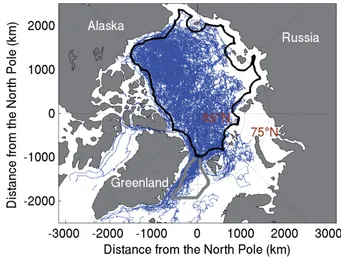
The sea ice drifting buoy dataset, provided by the Interna-tional Arctic Buoy Program (IABP), consists of approxi-mately 650 buoy tracks recorded from January 1979 to De-cember 2008. These ice drifters are dropped every year at the end of winter, mostly in April, and drift according to the ice motion. Their positions are tracked by GPS receivers or Argos transmitters with a position uncertainty of the or-der of 100 m and 300 m, respectively. The raw buoy posi-tions are irregularly sampled through time. Thus, in order to get a regular sampling, the buoy positions provided by the IABP result from a cubic interpolation of the raw positions with a 3 h time re-sampling (see the IABP documentation at http://iabp.apl.washington.edu/data.html for further details). This interpolation procedure acts as a low-pass filter, thus most likely reducing the position error around 100 m or be-low (Lindsay and Stern, 2003). Figure 1 shows all the buoy tracks on a polar stereographic map, where buoy locations are defined asxe1+ye2, wheree1ande2are two orthogonal unit vectors withe1being along the Greenwich meridian and
(x, y)=(0,0)at North Pole. 2.2 Oceanic buoy dataset
In order to get an example of the amplitude of inertial oscil-lations in the absence of sea ice, i.e. when the damping of oscillations is mainly due to the internal friction of the Ek-man layer without contribution from internal ice stresses, we consider trajectories of buoys drifting in the North Atlantic, along the northern Spanish coast (Fig. 2).
Fig. 1. Map of the Arctic Basin showing the buoy trajectories of the IABP dataset. The positions are sampled every 3 h from Jan-uary 1979 to December 2008 and plotted following a stereographic projection centered on the North Pole. The Laptev Sea is poorly covered by this dataset. The thick solid black and grey lines define the central Arctic Basin and the Fram Strait region, respectively.
This oceanic buoy dataset, provided by the SHOM (Ser-vice Hydrographique et Oceanographique de la Marine), consists of 4 buoy tracks (B239, B241, B242, B245). These buoys were deployed between 6 and 11 December 2006 in the framework of the CONtinental GAScogne (CONGAS) project (Le Cann and Serpette, 2009). The buoy positions were tracked by GPS receivers with a position uncertainty of the order of several tens of meters. The temporal sampling was regular, equal to 1 h. Thus, the buoy positions do not re-sult from any re-sampling or re-interpolation. Buoys B239 and B245 operated during 1 yr, whereas buoys B241 and B242 operated only 1 month. For each latitude (φ)–longitude (ϕ) buoy position, we define the orthogonal base (e′
1,e′2) of
this coordinate system asx(φ,ϕ)=xe′
1+ye′2using a Lambert
projection centered in the coordinatesφ=43◦andϕ=6◦.
3 Quantifying the magnitude of inertial oscillations
3.1 Observations
We analyze here several cases of inertial oscillations ob-served over an ice-free ocean or over sea ice.
15o W 12o
W 9oW 6oW 3oW 0o 38oN
40oN 42o
N 44o
N 46o
N 48o
N
φ
(degree)
ϕ
Spain
France
(degree)
Fig. 2. Map of the Atlantic Ocean showing the oceanic buoy trajec-tories deployed during the Congas project. The positions are sam-pled every 1 h and plotted following a Lambert projection.
(green boxes in Fig. 3a), before a new storm or moving front can trigger new inertial oscillations.
We compute the ux(x,˜ y,˜ t )˜ (along the x-axis) and uy(x,˜ y,˜ t )˜ (along the y-axis) speeds as follows:
ux(x,˜ y,˜ t )˜ =(x(t+1t )−x(t ))/1t
uy(x,˜ y,˜ t )˜ =(y(t+1t )−y(t ))/1t (3)
with1t=1 h and where the mid-pointsx˜,y˜ andt˜are de-fined asx˜=(x(t+1t )+x(t ))/2,y˜=(y(t+1t )+y(t ))/2 and t˜=((t+1t )+t )/2. The Fourier transform Uˆb(ω) of the buoy velocitiesuxanduyfor a selected buoy trajectory, which starts at timet0and ends at timetend, is defined as
ˆ Ub(ω)=
1
N tendX−1t
t=t0
e−iωt(ux(x,˜ t )˜ +iuy(y,˜ t ))˜ (4)
whereN is the number of velocity samples along the trajec-tory andω=2πf. This vectorial Fourier transform distin-guishes negative and positive frequencies: peaks atf <0 and
f >0 are associated with clockwise and counter-clockwise displacements, respectively.
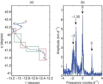
Figure 3b shows the Fourier spectrum | ˆUb(ω)| of the buoy velocities associated with the trajectory plotted in Fig. 3a. The Fourier transform reveals a peak of mag-nitude 5.2 km day−1 at the inertial oscillation frequency (f0≈ −1.35 cycles day−1 using the average latitude φ= 1/NPtφ (t )≈42◦in Eq. 1). This peak corresponds to the component of the buoy motion associated with the Coriolis force. The peak at f =0 represents the advective compo-nent of the buoy motion. Finally, the two peaks observed at
f = −2 cycles day−1andf =2 cycles day−1are associated with a semi-diurnal tidal oscillation. Unlike the inertial oscil-lation, the tidal oscillation does not rotate and the associated peak is therefore observed at positive and negative frequen-cies.
−13.2 −13 −12.8−12.6−12.4−12.2 41
41.2 41.4 41.6 41.8 42 42.2 42.4 42.6
φ
(degree)
−40 −2 0 2 4
1 2 3 4 5 6 7
Frequency (cycles.d−1)
Amplitude (km.d
−1
)
(b) (a)
0
2 −2
ϕ(degree)
−1.35
Fig. 3. (a) 1 month sample of the trajectory of buoy B245 (25 May to 25 June 2007). The trajectory is plotted in latitude-longitude co-ordinates. Its beginning is marked by the red circle. The red and green boxes outline periods with strong and low cycloidal loop ac-tivity, respectively. (b) Fourier spectrum of the buoy velocity. The velocity is computed following Eq. (3) with1t=1 h.
We now consider IABP ice drifters. A buoy moving in free drift, i.e. fixed on an ice floe that drifts according to wind and ocean currents alone, hence without any mechanical interac-tion with other ice floes, is expected to oscillate in a way similar to e.g. the oceanic B245 buoy of Fig. 3 when sub-jected to similar forcing conditions, although another source of damping of the oscillations might come from the friction between the ice bottom and the ocean surface.
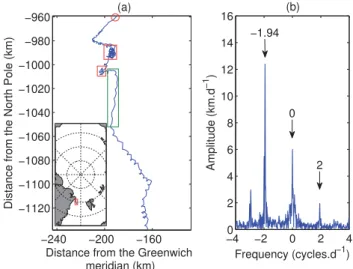
Figure 4a shows an IABP buoy trajectory within the Fram Strait during the summer period, where ice is highly fragmented and loosely packed. The clockwise-cycloids are clearly visible. We observe bursts in the inertial oscillation intensity (red rectangles) followed by a period of decaying intensity (green rectangle).
−240 −200 −160 −1120
−1100 −1080 −1060 −1040 −1020 −1000 −980 −960
Distance from the Greenwich meridian (km)
Distance from the North Pole (km)
−40 −2 0 2 4
2 4 6 8 10 12 14 16
Frequency (cycles.d−1)
Amplitude (km.d
−1
)
−1.94
0
2
(a) (b)
Fig. 4. (a) 1 month sample of the trajectory of IABP buoy 1897 (30 August to 30 September 1987). The location of the buoy is indicated by the red box in the inset of Fig. 4a. The red boxes show periods when cycloidal loops are best observed, whereas the amplitude of the loops is much lower in the green boxes. (b) Fourier spectrum of the buoy velocity. The velocity is computed following Eq. (3) with 1t=3 h.
amplitude of the peak at the inertial frequencyf0 is likely to represent the inertial component of the buoy motion. For example, in Fig. 4b, the tidal oscillation generates a small peak atf =2 cycles day−1, which means that most of the amplitude of the peak observed atf0comes from the inertial oscillation of the buoy.
We now consider a buoy tethered to a strongly cohesive multi-year ice pack: the internal stress term of the momen-tum equation (Eq. 2) is then expected to dominate over any external forcing, including the Coriolis force. Consequently, the inertial oscillations that might be generated by storms or moving fronts are immediately damped and thus not visible. Figure 5a shows an example of such a trajectory within the multi-year ice pack at the end of winter. The cycloids seen in Fig. 4a do not appear anymore and the Fourier spectrum plotted in Fig. 5b does not show any peak at the inertial fre-quencyf0. Conversely, we can notice that Kwok et al. (2003) found significant oscillations in the same region but in a dif-ferent time period. This points out the temporal variability in the strength of inertial oscillations, which may depend on both the storm activity and the sea ice state. In the following, a simple method is proposed to quantify the strength of iner-tial oscillations. Then, performing statistics on this quantity will allow us to interpret space and time variabilities in terms of dissipation of energy through mechanical processes that takes place within sea ice.
−60 −40 −20 0
520 540 560 580 600 620
Distance from the 180e meridian (km)
Distance from the North Pole (km)
−40 −2 0 2 4
0.5 1 1.5 2 2.5 3 3.5
Frequency (cycles.d−1)
Amplitude (km.d
−1
)
(a) (b)
Fig. 5. (a) 1 month sample of the trajectory of buoy 12825 (20 April to 21 May 1992). The location of the buoy within the Arctic Basin is indicated by the red box in the inset of Fig. 5a. (b) Fourier spectrum of the buoy velocity. The velocity is computed following Eq. (3) with1t=3 h.
3.2 Methodology
We now define a parameterM that quantitatively accounts for the time-dependent inertial oscillation magnitude.
The cycloids observed in the trajectories (Sect. 3.1) result from the superposition of an advection (f =0) and a rota-tion at the inertial frequency (f =f0). In Figs. 3 and 4, the red boxes show parts of the trajectories characterized by cy-cloidal loops: these loops indicate that the rotation velocity is larger than the advection velocity. In contrast, no full loops are observed within the green boxes, showing that the rota-tion velocity is lower than the advecrota-tion velocity. Lepparanta (2004, p. 157) proposed a simple ratio of cycloidal rotation velocity over the advection velocity to qualitatively estimate the strength of inertial oscillations.
We here propose to evaluate in a quantitative way the time-dependent oscillation magnitude using the Fourier spectrum at the inertial frequencyf0. Since inertial oscillations are best quantified by means of a spectral analysis, we here perform such an analysis on a sliding time window. This will enable us to define a time-varying quantity M that measures how inertial oscillations evolve with time as a buoy drifts. For a given buoy location defined by the coordinates (xpst,ypst,
tpst), where “pst” stands for “present”, we define a Gaussian window functiongpst(t )centered ontpstwith a characteristic duration of the order of several inertial time periods:
gpst(t )=exp −
(t−tpst)2 2(nTo)2
!
(5)
probe the inertial time scale, since it corresponds to 3 days, and short enough to properly measure rapid time variations in the inertial oscillation magnitude. Thus, 24 data points within which about half the points carry significant weight are used to compute Fourier transform calculations.
Gaps (missing data) are present in the IABP buoy records. Their duration varies from one sample every few hours (i.e. a time interval of 6 h between successive positions) to several weeks. Therefore, we introduce in our calculations a selection condition such that no gap of data is allowed for values oft that verifygpst(t ) > P, where we setP =0.01. NoMvalue is thus computed at timetpstif one or more sam-pling timet verifying this later condition is lacking. More-over, since missing data even occurring far fromtpst(i.e. at values oft such thatgpst(t ) < P) can play a non-negligible role on the Fourier transforms, the Gaussian of Eq. (5) is trun-cated at±1.5 days fromtpst.
Under these conditions, we can compute 1.3×10⁶M val-ues from the IABP dataset, which represents 83 % of the total number of observations available.
We then compute the velocityWpst(t )as follows:
Wpst(t )=Ub(t )gpst(t ) (6)
whereUb(t )=ux(t )e1+uy(t )e2.
We compute the normalized Fourier spectrum at timetpst of the velocity time seriesWpst(t )at the inertial frequency
f0, wheref0is made to vary according to the buoy latitude (Eq. 1), as
ˆ
Wpst(f0)=1t
tend
X
t=t0
(ux(t )+iuy(t ))gpst(t )e−iω0t (7)
whereω0=2πf0andt0andtendare the starting and ending times of the trajectory. This value is likely to represent the amplitude of the inertial oscillations. We further normalize it in order to define a non-dimensional parameterMthat mea-sures the magnitude (still attpst) of the inertial oscillation:
M=| ˆWpst(f0)|
1.27 × 4
π Wpst
(8) where
Wpst= 1 1.27
tend
X
t0
dt|Wpst(t )|. (9)
is the (current, at timetpst) mean magnitude of the drift ve-locity, and the value 1.27 is equal toRtend
t0 gpst(t )dt. 3.3 Application to the buoy trajectories
Figure 6 shows the values ofMcomputed using the different trajectories plotted in Sect. 3.1. LargeMvalues are obtained for the oceanic buoy trajectory plotted in Fig. 3, with an av-erage of 0.56. For the ice drifter of Fig. 4, we also get large
M values with an average of 0.8: theM >1 values are all associated with cycloidal loops observed in Fig. 4a (red rect-angles), followed by their decay as characterized by a de-crease ofM(green rectangles). In contrast, for the ice drifter of Fig. 6c, theMvalues are much lower: the meanMvalue over the time period is only equal to 0.13, illustrating the rel-ative absence of inertial loops.
As the raw buoy positions of the IABP ice drifters dataset are irregularly sampled through time, then interpolated (cu-bic interpolation) and re-sampled at a regular 3 h interval, we investigated the effect of this procedure on the values ofM
computed for the IABP dataset. To do so, we artificially de-graded the oceanic buoy dataset, which samples buoys po-sitions every hour, by randomly removing a given % of raw positions. A cubic interpolation followed by a re-sampling at 3 h is then performed on the degraded dataset, as done for IABP data, and the associatedMvalues (notedMD) are re-computed (Fig. 7). The cubic interpolation alone, i.e. with-out degrading the raw data, has almost no influence on M
(Fig. 7a). In Fig. 7b, we can see that the deviation of the
MDtime series from theMtime series becomes visible only when more than 50 % of the raw buoy positions are missing. For 50 % of missing data, the error on individualMvalues is lower than 5 %. More importantly, as we focus in the follow-ing onMvalues averaged over trajectories, the departure of averagedMDvalues from the average Mvalue for increas-ing missincreas-ing data ratios is shown in Fig. 7c. AverageMD val-ues do not deviate significantly from the averageMvalue for missing data ratios up to 60 %, which corresponds to an aver-age time sampling of about 02:50 h and a time sampling max-imum gap of about 6 h. Thus, for sampling times lower than these threshold values, we can consider that the computed
Mvalues are not affected by an irregular sampling through time. While not shown here, similar results have been ob-tained by considering ice drifters initially regularly sampled at 1 h during the TARA field campaign (Gascard et al., 2008). This indicates the robustness of IABP interpolation proce-dure coupled to our estimation of the amplitude of inertial oscillations.
These examples demonstrate that the parameterM is ap-propriate to quantify the inertial oscillation magnitude. Small average values ofM(say lower than 0.2) correspond to buoy trajectories within a strongly cohesive ice pack, while large values ofM(say greater than 0.6) correspond to buoy trajec-tories that we can consider to be nearly in free drift condition.
4 Analysis of 30 yr of IABP data
05/250 05/01 06/08 06/15 06/22 0.25
0.5 0.75 1 1.25
Date
M value
(a)
07/30 08/04 08/09 08/14 08/19 08/24 08/290
0.25 0.5 0.75 1 1.25
Date
M
va
lue
(b)
04/20 04/25 04/30 05/05 05/10 05/15 05/200
0.25 0.5 0.75 1 1.25
Date
M
va
lue
(c)
Fig. 6.Mvalues for (a) the trajectory of the oceanic buoy 255 plotted in Fig. 3a, (b) the trajectory of the ice-tethered buoy 1897 plotted in Fig. 4a and (c) the trajectory of the buoy 12825 plotted in Fig. 5a. The red and green rectangles respectively correspond to those shown in Figs. 3 and 4.
05/250 05/01 06/08 06/15 06/22 0.25
0.5 0.75 1 1.25
Date
M
va
lue
(a)
05/250 05/01 06/08 06/15 06/22 0.25
0.5 0.75 1 1.25
Date
M
va
lue
0.05 0.15 0.25 0.35 0.45 0.55
(b)
0 0.1 0.2 0.3 0.4 0.5 0.6 0.7 0.8 0.9 1 0
0.1 0.2 0.3 0.4 0.5 0.6
Ratio of missing data
Average M−value
(c)
Fig. 7. (a)Mvalues for the trajectory of the oceanic buoy 255 plotted in Fig. 3 (raw data: blue line, same as Fig. 6a) and the trajectory obtained after a cubic interpolation and a 3 h resampling of the raw positions (red line). (b)MD time series computed from the degraded datasets of missing data ratio varying between 0 and 60 % (the red line is the same as in a). (c)MDvalues averaged over the whole trajectory (1 month) as a function of the missing data ratio. 20 realisations have been done at each given value of missing data ratio. The grey dashed line shows the average rawMvalue, equal to 0.56.
in external forces (strong wind), which then decay due to ki-netic energy dissipation within the Ekman layer or friction that takes place at the ice/water interface, or due to internal ice stresses. Therefore, more frequent and stronger storms over the years should imply larger M values on average. Cyclonic activity over the Arctic Ocean shows a maximum during summer that could partly explain an annual cycle of the inertial oscillation magnitude (Serreze and Barrett, 2008) (see below). On the other hand, no significant trend in cy-clonic activity has been found over the last 50 yr (Serreze and Barrett, 2008). Similarly, the average wind speed over the Arctic Basin, as estimated from the ERA-40 reanalysis dataset, does not show any significant trend over the period 1979–1999 (Rampal et al., 2009).
4.1 Seasonal variation
In this section, we computeM for buoys located within the central Arctic Basin, as delimited by the thick black line in Fig. 1, and then investigate intra-annual (monthly) variations by groupingMvalues into monthly periods, i.e. one average monthly valueM for all theMvalues occurring in January,
whatever the calendar year, etc. The central Arctic is here de-limited by all buoy positions lying further than 150 km away from the coasts and the Fram Strait. This way, we skip from the analysis buoys possibly stuck on fast ice.
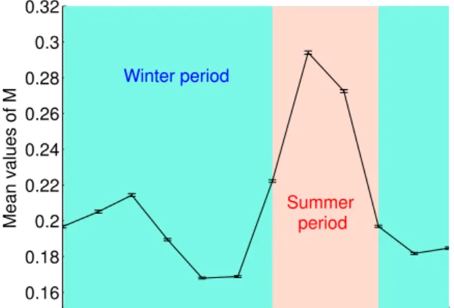
Figure 8 shows the monthlyM value averaged over the 30 yr of record. To estimate the associated error bars, we checked using a bootstrap method (Rampal et al., 2009) that the standard deviation1Mindeed varies as√M
Jan Feb Mar Apr May Jun Jul Aug Sep Oct Nov Dec 0.16
0.18 0.2 0.22 0.24 0.26 0.28 0.3 0.32
Month of the year
Mean values of M
Winter period
Summer period
Fig. 8. Average annual cycle in theMvalues. The average is per-formed considering the central Arctic Basin buoy dataset. The error bars show the deviation1Mfrom the averageM value estimated using the central limit theorem and computed as 1M=√M
NM, whereNMis the number ofMvalues used to calculate the monthly meanM. Here,NM ranges from a minimum of 6.4×10⁴in Febru-ary to a maximum of 1.1×10⁵in May.
Mvalue in May. Being thinner and less concentrated in sum-mer, sea ice is less cohesive and more deformable during this time period. This leads, on average, to a lower damping of the inertial oscillations, and therefore largerMvalues. However, we cannot exclude that a stronger cyclonic activity during summer (Serreze and Barrett, 2008) could reinforce the an-nual cycle described by the averageMvalues by triggering more oscillations.
4.2 Spatial pattern
The question arises as to whether the seasonal changes in the
M values evidenced in the previous section can be associ-ated with a spatial pattern. In this section, we select values of M associated to buoys located within the central Arctic Basin and within the Fram Strait (thick black and grey lines in Fig. 1). From theses values, we build a seasonalMdataset by separating theMvalues computed in winter, i.e. all the
M values recorded for all the 30 winter seasons, from the
Mvalues computed in summer. The seasonal spatial patterns ofMfor both seasons are plotted in Fig. 9. The spatially av-eragedMvalue, denoted M(Xj, Yj), is computed for each
grid pointj of coordinates (Xj,Yj) as
M(Xj, Yj)=P 1 iwij(xi, yi)
X
i
wij(xi, yi)Mi(xi, yi) (10)
where the summation is performed over all the buoy posi-tions(xi, yi)contained in a circle of radiusL=400 km
cen-tered on the coordinates (Xj,Yj). The weight wij(xi, yi)is
defined as
wij(xi, yi)=e−d2/2L2 (11)
where d= q
(xi−Xj)2+(yi−Yj)2 is the distance buoy
position(xi, yi)and the grid point(Xj, Yj).
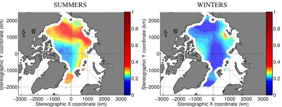
The patterns observed in Fig. 9 are, at least qualitatively, consistent with the observed distribution of the sea ice thick-ness (Kwok and Rothrock, 2009) and concentration (http: //nsidc.org/data/seaice/index.html) (Comiso, 1990, updated 2012). In summer, largeMvalues are observed at the edge of the basin in the Beaufort, Chukchi and Laptev seas, i.e. in re-gions where the multi-year ice cover has been progressively disappearing during the last decade (Maslanik et al., 2011). On the contrary, small values of M can be observed along the Canadian coasts, where the average ice thickness is at its maximum (Kwok and Rothrock, 2009). Sea ice behaves more as a strongly cohesive plate in this region, unsensitive to the Coriolis force. This zone corresponds to the multi-year ice still remaining nowadays. Large values ofMare also ob-served south of Fram Strait, which is consistent with the buoy trajectory plotted in Fig. 4a, which we discussed in Sect. 3.1. In contrast, the winter pattern does not reveal any particu-lar structure within the basin. The values of M are small over the whole basin, except relatively largerMvalues com-puted north of Canadian coasts. These largerMvalues could be attributed to buoys drifting along the “Circumpolar flaw lead” that consists of a sheared, thus highly fragmented, zone (Lukovich et al., 2011).
To further test the link between the state of the sea ice cover and its cohesiveness, as expressed by the am-plitude of the inertial oscillations, we perform a correla-tion analysis between the M values and the open water concentration 1−α, where α is the sea ice concentration dataset collected by NSIDC (http://nsidc.org/data/seaice/ index.html) (Comiso, 1990, updated 2012). This dataset has a spatial resolution of 25 km and consists of ice concentration values sampled every two days from 1979 to 1987 (SMMR), and every day since 1987 (SSM/I). For each value ofM, we search for the corresponding value of open water concentra-tion as the closest sample in time and space: a 1−αvalue is associated with a givenMvalue if we can find, for the same day of record, within one day during the period 1979–1987, a sample that is closer than 25 km. The corresponding corre-lation coefficientRis equal to 0.245(±0.002). This positive correlation is statistically significant asR is more than 120 times greater than the standard deviation obtained in the null hypothesis at no correlation (numerically computed by ran-domly reshuffling theMand 1−αvalues). This is consistent with stronger oscillations characteristic of a less compact sea ice cover.
SUMMERS
−3000 −2000 −1000 0 1000 2000 3000 −2000
−1000 0 1000 2000
Stereographic X coordinate (km)
Stereographic Y coordinate (km)
0 0.2 0.4 0.6 0.8 1
WINTERS
−3000 −2000 −1000 0 1000 2000 3000 −2000
−1000 0 1000 2000
Stereographic X coordinate (km)
Stereographic Y coordinate (km)
0 0.2 0.4 0.6 0.8 1
Fig. 9. Spatial pattern of inertial oscillation magnitude within the Arctic Basin in summer (left) and in winter (right). These two fields are computed from the seasonalMdataset. A spatially averaged value ofMvalues, denotedM, is computed following Eq. (10) for each point of a 25 km resolution grid. The graphic representation is a linear interpolation of the griddedMvalues. In order to not represent regions with little data, anMvalue at a given grid point is plotted only if its associated weight is greater than a minimum value we arbitrarily set to 1000.
for each month of the year, over the 30 yr of record. While not plotted here, the annual variation of the correlation co-efficient is in phase with the annual cycle ofM plotted in Fig. 8: the correlation is larger in summer. The correlation co-efficient is equal to 0.350(±0.005)in August, which means that theMvalues are spatially correlated with the associated open water concentration values. In winter, the correlation is much less significant, which can be understood by the fact that, during this period, the sea ice concentrations are equal to 1 almost everywhere within the basin and therefore show very little fluctuations.
Here, all the computed coefficients of correlation remain small. This suggests that other factors than the ice concentra-tion control theMvalues: we expect both the variability in wind forcing materialized by storm activity and the ice thick-ness to significantly depress the correlation betweenM and 1−α. We will see in Sect. 4.3.2 that the correlation between
Mand 1−αis much improved when setting free of the influ-ence of wind forcing variability, i.e. by considering averaged
Mand 1−αvalues.
4.3 Multi-annual variation
We have shown so far that theMparameter is a useful proxy for the cohesiveness of the cover and, consequently, the level of internal stresses. We now analyze whether theMvalues have changed over the last three decades owing to a change in ice conditions.
4.3.1 Mtime series
In this section, we use the central Arctic buoy dataset. The temporal sampling of the IABP buoy dataset is heteroge-neous, being characterized by variations of data density over the period. Most notably, a larger number of observations are available in the later years, as compared to the early 1980s
or during the late 1990s. To circumvent this problem, the evaluation of the multi-annual variation of M is done by equally binning theMvalues in time. The summer and win-ter datasets are both separately split into 10 successive bins, all containing the same number of observations. For each bin, an average value ofM, associated with an average value of time, is computed.
Figure 10 shows the time series M(t ) between January 1979 and December 2008 for the summer and winter sea-sons. The error in the averageM value is computed using a bootstrap method as explained in Rampal et al. (2009). The bootstrap method is performed individually for each bin, and the deviation from the mean 1M is represented by the er-ror bars. We see on both plots that the most prominent fea-ture is a significant increase of the inertial oscillation ampli-tude through time. A linear fit gives a positive trend equal to 1.19 (±0.34)×10−5yr−1(i.e. a 16.5 % increase per decade) for summer and 5.7 (±1.9)×10−6yr−1(i.e. a 11 % increase per decade) for winter. Thus, the increase of inertial oscilla-tions is relatively more marked in summer than in winter.
The use of GPS as the buoy positioning system has be-come more common since the end of the last century. As noted in Sect. 2.1, this system is more accurate than ARGOS positioning. We thus check whether the observed trend on the mean time seriesM(t )could be a spurious effect caused by reduced noise in recent years. To do so, noised mean time seriesMN(t )are built by computingMvalues on buoy
tra-jectories over which Gaussian noise is added. Because the increase in the average M(t ) values is particularly marked from the beginning of the 21 century, Gaussian noise is only added to buoy trajectories recorded during the period 2002– 2008. For each IABP position (xb,yb) of buoy trajectories recorded from the year 2002 onwards, we define a noised buoy position (xeb,yeb) asxeb=xb+δxandyeb=yb+δywhere
SUMMER
1975 1980 1985 1990 1995 2000 2005 2010 0.2
0.25 0.3 0.35 0.4
Date
Average M value
Period 1 Period 2 (a)
WINTER
1975 1980 1985 1990 1995 2000 2005 2010 0.14
0.16 0.18 0.2 0.22 0.24 0.26
Date
Average M value
Period 1 Period 2 (b)
Fig. 10. Time seriesM(t )from January 1979 to December 2008 computed using (a) the summer dataset and (b) the winter dataset. For each season, the dataset is equally split into 10 bins over which the average is computed. One bin corresponds to approximately 3.1×10⁴Mvalues in summer and 8.0×10⁴Mvalues in winter. The horizontal lines associated with each data point indicate the time period associated with each bin. Vertical lines are error bars computed from a bootstrap method. Bold lines are linear fits: the trends are 1.19 (±0.34)×10−5yr−1 (i.e. 16.5 % increase per decade) for summer and 5.7 (±1.9)×10−6yr−1(i.e. 11 % increase per decade) for winter.
Gaussian distribution with a standard deviationσ. Figure 11 shows realizations of mean time series MN(t ) built using
σ=300 m and σ=1000 m, along with the IABP time se-riesM(t ), as in Fig. 10. From the year 2002, the mean time seriesMN(t )deviate fromM(t ), showing that noise on the
buoy positions has an influence on the parameterM. How-ever, almost systematically, values ofMN(t )are larger than M(t ), showing that noise most generally acts to increase the
Mvalues rather than to decrease them.
This can be explained as follows: noise increases the am-plitude of the Fourier spectrum at high frequencies. This has two competing consequences: (i) the norm of the drift ve-locity Wpst slightly increases, which tends to decrease M (see Eq. 9); and (ii) the amplitude at the inertial frequency
ˆ
Wpst(f0)is increased, which tends to increase M. The sec-ond effect is particularly marked when the inertial motion (so,M) is small, and, most of the time, dominates over the first effect, so thatMis increased by noise. Consequently, the evolution observed in Fig. 10 is not the consequence of pos-sible reduced position noise in recent years, as the difference between the periods 1979–2001 and 2002–2008 would have been even larger if the level of noise had remained the same over the entire record. In other words, the observed trend in
M(t )is most likely an underestimation of the multi-annual evolution of the inertial oscillation magnitude.
The same is also true for the annual cycle (Fig. 7): as the effect of noise is stronger for lowMvalues, winterMvalues are, in average, more overestimated than summerMvalues.
In addition, Rampal et al. (2009) reported a significant (9 % per decade) increase of sea ice speeds in the Arctic Basin over the last three decades. Therefore, as increasing advection velocities act to decreaseM(Sect. 3.2), the multi-annual positive trend on the M values reported here most likely underestimates the associated decrease of the mechan-ical energy dissipation within the ice cover in the later years.
4.3.2 Evolution of spatial patterns
The previous section demonstrated a strong evolution of the average inertial oscillation amplitude, although it is more strongly marked in summer. We here analyze the spatial con-sequences of the observed multi-annual changes. To do so, we split the whole IABP buoy seasonal dataset into two pe-riods. A Student t-test performed on the winter and the sum-mer M(t )-time series in Fig. 10 shows that the most sig-nificant changing point occurs in 5 averagedM values out of the 10. More precisely, splitting the winter time series
{M1, M2, . . ., M10} into two distributions{M1, . . ., M5}and
{M6, . . ., M10}, the probability that these two distributions have the same mean is only 0.92 %. We have verified that this probability is indeed the lowest when splitting the time series just afterM5. Similarly, we find the same optimal change-point in summer, with an associated probability that the two distributions share the same mean equal to 0.42 %. This leads to define two distinct periods, with period 1 from 1979 to 2001 and period 2 from 2002 to 2008 (see Fig. 10). We can remark that, according to this periodic splitting, period 1 and period 2 contain the same number of observations, i.e. 5 bins each. As done in Sect. 4.2, the spatial patterns of theM val-ues for the summer and winter seasons associated with each period are shown in Fig. 12. As expected, the changes are stronger in summer. They affect most of the Arctic, but are more pronounced on the Siberian side: a drastic increase of the peripheral ice zone area is observed in the later years. Conversely, winter changes are milder north of Canada and Greenland, where the thickest multi-year ice can be found nowadays (Kwok and Rothrock, 2009).
To underline the link between the spatial repartition of
SUMMER
1980 1990 2000 2010
0.2 0.25 0.3 0.35
Date
Average M value
IABP σ=300m
σ=1000m
(a)
WINTER
1980 1990 2000 2010
0.15 0.2 0.25 0.3
Date
Average M value
σ=1000m
σ=300m
IABP (b)
Fig. 11. Influence of noise, prescribed on the positions of buoys, on the monthly mean time seriesM(t )for (a) the summer season and (b) the winter season. Gaussian noise, with a constant standard deviationσ, has been added to all buoy positions recorded since year 2002. Results for noised mean time seriesMN(t )(in yellow and green) forσ=300 m andσ=1000 m are compared with the IABP mean time seriesM(t ) as in Fig. 10.
1979-2001 SUMMERS
−3000 −2000 −1000 0 1000 2000 3000 −2000
−1000 0 1000 2000
Stereographic X coordinate (km)
Stereographic Y coordinate (km)
0 0.2 0.4 0.6 0.8 1
2002-2008 SUMMERS
−3000 −2000 −1000 0 1000 2000 3000 −2000
−1000 0 1000 2000
Stereographic X coordinate (km)
Stereographic Y coordinate (km)
0 0.2 0.4 0.6 0.8 1
1979-2001 WINTERS
−3000 −2000 −1000 0 1000 2000 3000 −2000
−1000 0 1000 2000
Stereographic X coordinate (km)
Stereographic Y coordinate (km)
0 0.2 0.4 0.6 0.8 1
2002-2008 WINTERS
−3000 −2000 −1000 0 1000 2000 3000 −2000
−1000 0 1000 2000
Stereographic X coordinate (km)
Stereographic Y coordinate (km)
0 0.2 0.4 0.6 0.8 1
Fig. 12. Spatial repartition ofMwithin the Arctic Basin in summer and winter computed using the seasonal dataset of the period 1979–2001 and the seasonal dataset of the period 2002–2008. An average mean value ofM, denotedM, is computed following Eq. (10) for each node of a 25 km resolution grid. The smoothing parameterLis equal to 400 km. In order to not represent regions with little data, anMvalue at a given grid point is plotted only if its associated weight is greater than a minimum value we arbitrarily set to 1000.
here, since they correspond to 1−αvalues very close to 0 over the whole Arctic Basin. Sea ice concentration values are sampled at buoy positions, as done in section 4.2, and averaged similarly toMvalues, i.e. following Eq. 10. Com-mon features evidenced byM in Fig. 9 (left) and Fig. 12
SUMMERS 1979-2001
−2000 −1000 0 1000 2000 −2000
−1000 0 1000 2000
Stereographic X coordinate (km)
Stereographic Y coordinate (km)
0 0.2 0.4 0.6 0.8 1
SUMMERS 2002-2008
−2000 −1000 0 1000 2000 −2000
−1000 0 1000 2000
Stereographic X coordinate (km)
Stereographic Y coordinate (km)
0 0.2 0.4 0.6 0.8 1
Fig. 13. Spatial repartition of open water concentration within the Arctic Basin in summer computed using the seasonal dataset of the period 1979–2001 and the seasonal dataset of the period 2002–2008. An average mean value of open water concentration, denoted 1−α, is computed following Eq. (10) for each node of a 25 km resolution grid. The smoothing parameterLis equal to 400 km. In order to not represent regions with little data, an open water concentration value at a given grid point is plotted only if its associated weight is greater than a minimum value we arbitrarily set to 1000.
from period 1 to period 2 is also similar to the one observed onM, materialized by a slight migration of the pack zone to-ward the south, and an increase of the peripheral zone area, materialized by larger open water concentration values. The correlation coefficient computed between M values shown in Fig. 12 and values of 1−αis equal to 0.57 for period 1 and 0.80 for period 2. These correlation coefficients are much larger than the one obtained in section 4.2. This is explained by the fact that averageM and 1−αvalues are considered here prior to compute the correlation coefficient, removing like this the influence of wind forcing activity in the variabil-ity ofM. Thus, we expect the discrepancies that still remain here betweenM and 1−α to be mostly due to changes in ice thickness and ice degree of fragmentation. The respective role of ice concentration, ice thickness and ice degree of frag-mentation on the inertial oscillation amplitude is thoroughly examined in Gimbert et al. (2012).
4.3.3 Is the observed evolution from the IABP buoy dataset representative of the whole Arctic Basin?
In the two previous sections, care was taken to remove the effect of temporal heterogeneities in the IABP buoy dataset. However, the IABP buoy dataset is spatially heterogeneous: changes in the spatial sampling by the buoys could affect the overall trend. In order to check whether the results reported in Fig. 10 truly indicate a significant increase of theM val-ues, we investigate whether this trend could be an artefact of changes in spatial sampling.
Following the procedure described in Rampal et al. (2009) for ice velocities, we formulate a null hypothesis: in this hy-pothesis, there exists no temporal changes in M-maps over the year, but the effect at spatially sampling these maps in
different ways at different periods will cause the M-time series to evolve with time. To construct these M-maps, we consider any buoy position associated with a givenMvalue and recorded at a given year and a given season. For such a position, we compute the meanM0value for summer, re-spectively winter, by considering all theM values recorded in summer, respectively winter, and whatever the year, con-tained within a circle of radiusL=200 km, using Eq. (10). This mean value is therefore year-independent, and corre-sponds to our null hypothesis of no inter-annual changes. Then, we calculate our null-hypothesisM0time series as the mean of the summer, respectively winterMvalues, using the same bins as in Fig. 10. Any inter-annual variation observed in the time seriesM0(t )could only be explained by changes in the spatial sampling rather than by an actual, global trend: for example, a positive trend would be explained if IABP buoy had a tendency to sample regions associated with large
Mvalues more often in the later years as compared to earlier years.
SUMMER
1975 1980 1985 1990 1995 2000 2005 2010 0.2
0.25 0.3 0.35 0.4
Date
Average M value
(a)
WINTER
1975 1980 1985 1990 1995 2000 2005 2010
0.14 0.16 0.18 0.2 0.22 0.24 0.26
Date
Average M value
(b)
Fig. 14. Mean time seriesM(t )(a) in summer (red) and (b) in winter (blue), as in Fig. 10 andM0(t )(black lines), resulting from the null hypothesis. The best linear fits are also plotted, showing that changes in spatial sampling only account for a small fraction of the observed trend.
5 Conclusions
From the IABP ice drifter trajectories recorded between 1979 and 2008, we analyzed the average amplitude of inertial os-cillations over the Arctic sea ice cover. To do so, we defined a non-dimensional parameterM that quantifies the magni-tude of inertial oscillations relative to advection motion along the trajectories. For a sea ice cover of low concentration, con-stituted from a loose floe field moving nearly in free drift, inertial motions and M values are large. On the reverse, a highly cohesive sea ice pack, characterized by strong inter-nal stresses, is expected to be associated with lowMvalues. From appropriate averaging of this 30-yr dataset at different space or time scales, we have shown the following:
(i) TheMvalues describe an annual cycle with a minimum reached in May and a maximum in September, in a qual-itative agreement with the corresponding annual cycles of sea ice extent (Comiso et al., 2008), concentration, thickness (Rothrock et al., 2008; Kwok and Rothrock, 2009), advection velocity and deformation rates (Ram-pal et al., 2009).
(ii) The spatial pattern of M over the Arctic Basin is in agreement with the sea ice thickness and concentration patterns. LowMvalues are observed in western Arctic, whereas large values are observed within a peripheral zone (Beaufort Sea, eastern Arctic) and south of Fram Strait.
(iii) A significant increase of average values of M is ob-served from 1979 to 2008. This increase, although more marked in summer, is observed in both seasons and is associated with the reduction of the thick, multi-year ice zone in recent years.
From the expected link between the magnitude of the oscillations and the degree of consolidation of the ice cover (McPhee, 1978; Colony and Thorndike, 1980; Geiger
and Perovich, 2008), we believe that point (iii) is a signa-ture of the mechanical weakening of the Arctic sea ice cover in recent years. However, one may argue from the momen-tum balance of sea ice (see Eq. (2)), that this strengthen-ing of inertial motion might simply and more directly result from the observed thinning of the cover, i.e. a reduction of ice mass per unit area. In addition, this evolution could, to some extent, be the result of a modification of vertical pen-etration of turbulent momentum within the ocean boundary layer. In Gimbert et al. (2012), we have shown, from a sim-ple ocean-sea ice cousim-pled dynamical model, that these two explanations cannot fully account for the evolution of iner-tial motion in the Arctic, which actually reveals a genuine mechanical weakening, through an associate decrease of the sea ice internal friction magnitude, of the cover at the basin scale. Such mechanical weakening has (will have) strong consequences in terms of ice drifting speeds, deformation rates, export (Rampal et al., 2009) and therefore on mass bal-ance (Rampal et al., 2011).
Acknowledgements. This study owes much to a suggestion by Stephane Roux. We thank the IABP for the availability of their buoy dataset as well as the SHOM laboratory for having provided us the oceanic buoys trajectories. We also thank Pierre Rampal and Neige Calonne for earlier work on this topic and helpful discussions. We thank the two anonymous reviewers and the associate editors for their constructive comments.
Edited by: R. Lindsay and W. Lipscomb
References
Aranson, I. and Tsimring, L.: Patterns and collective behavior in granular media: theoretical concepts, Rev. Mod. Phys., 78, 641– 692, 2006.
Colony, R. and Thorndike, A.: The horizontal co-herency of the motion of summer Arctic sea ice, J. Phys. Oceanogr., 10, 1281–1289, doi:10.1175/1520-0485(1980)010<1281:THCOTM>2.0.CO;2, 1980.
Comiso, J.: Bootstrap sea ice concentrations from NIMBUS-7 SMMR and DMSP SSM/I (January 1979 to December 2008), edited by: Maslanik, J. and Stroeve, J., Digital media, NSIDC, Boulder, Colorado, USA, 1990, updated 2012.
Comiso, J. C., Parkinson, C. L., Gersten, R., and Stock, L.: Acceler-ated decline in the Arctic sea ice cover, Geophys. Res. Lett., 35, L01703, doi:10.1029/2007GL031972, 2008.
D’Asaro, E. A., Eriksen, C. C., Levine, M. D., Niiler, P., Paul-son, C. A., and Meurs, P. V.: Upper-ocean inertial currents forced by a strong storm, Part I: Data and comparisons with linear theory, J. Phys. Oceanogr., 25, 2909–2936, doi:10.1175/1520-0485(1995)025<2909:UOICFB>2.0.CO;2, 1995.
Ekman, W.: On the influence of the earth’s rotation on ocean-currents., Ark. Mat. Astron. Fys., 2, 1–52, 1905.
Gascard, J., Festy, J., le Goff, H., Weber, M., Bruemmer, B., Offer-mann, M., Doble, M., Wadhams, P., Forsberg, R., Hanson, S., Sk-ourup, H., Gerland, S., Nicolaus, M., Metaxian, J., Grangeon, J., Haapala, J., Rinne, E., Haas, C., Heygster, G., Jakobson, E., Erko, T., Wilkinson, J., Kaleschke, L., Claffey, K., Elder, B., and Bottenheim, J.: Exploring Arctic transpolar drift during dramatic sea ice retreat, EOS, 89, 21–22, 2008.
Geiger, C. and Perovich, D.: Springtime ice motion in the Western Antarctic Peninsula region, Deep-Sea Res. Pt. II, 55, 338–350, 2008.
Gill, A. E.: On the behavior of inertial waves in the wakes of storms, J. Phys. Oceanogr., 14, 1129–1151, 1984.
Gimbert, F., Jourdain, N. C., Marsan, D., Weiss, J., and Barnier, B.: Recent mechanical weakening of the Arctic sea ice cover as re-vealed by larger sea ice inertial oscillations, J. Geophys. Res., 117, C00J12, doi:10.1029/2011JC007633, 2012.
Haas, C., Pfaffling, A., Hendricks, S., Rabenstein, L., Etienne, J., and Rigor, I.: Reduced ice thickness in Arctic transpolar drift favors rapid ice retreat, Geophys. Res. Lett., 35, L17501, doi:10.1029/2008GL034457, 2008.
Hunkins, K.: Inertial oscillations of fletcher’s ice island (T-3), J. Geophys. Res., 72, 1165–1174, doi:10.1029/JZ072i004p01165, 1967.
Hutchings, J., Heil, P., Steer, A., and Hibler III, W. D.: Sub-synoptic scale spatial variability of sea ice deformation in the West-ern Weddell sea during early summer, J. Geophys. Res., 117, C01002, doi:10.1029/2011JC006961, 2012.
Kwok, R. and Rothrock, D. A.: Decline in Arctic sea ice thickness from submarine and icesat records: 1958–2008, Geophys. Res. Lett., 36, L15501, doi:10.1029/2009GL039035, 2009.
Kwok, R., Cunningham, G. F., and Hibler III, W. D.: Sub-daily sea ice motion and deformation from RADARSAT observations, Geophys. Res. Lett., 30, 2218, doi:10.1029/2003GL018723, 2003.
Kwok, R., Pedersen, L. T., Gudmandsen, P., and Pang, S. S.: Large sea ice outflow into the nares strait in 2007, Geophys. Res. Lett., 37, L03502, doi:10.1029/2009GL041872, 2010.
Lammert, A., Brummer, B., and Kaleschke, L.: Observation of cyclone-induced inertial sea-ice oscillation in fram strait, Geo-phys. Res. Lett., 36, L10503, doi:10.1029/2009GL037197, 2009. Le Cann, B. and Serpette, A.: Intense warm and saline upper ocean inflow in the southern bay of biscay in autumn-winter 2006–2007, Cont. Shelf Res., 29, 1014–1025, doi:10.1016/j.csr.2008.11.015, 2009.
Lepparanta, M.: The drift of sea ice, Springer, 2004.
Lepparanta, M., Oikkonen, A., Shirasawa, K., and Fuka-machi, Y.: A treatise on frequency spectrum of drift ice velocity, Cold Reg. Sci. Technol., 76–77, 83–91, doi:10.1016/j.coldregions.2011.12.005, 2012.
Lindsay, R. W. and Stern, H. L.: The radarsat geophysical processor system: quality of sea ice trajectory and deformation estimates, J. Atmos. Ocean Tech., 20, 1333–1347, 2003.
Lindsay, R. W., Zhang, J., Schweiger, A., Steele, M., and Stern, H.: Arctic sea ice retreat in 2007 follows thinning trend, J. Climate, 22, 165–175, 2009.
Lukovich, J. V., Babb, D. G., and Barber, D. G.: On the scal-ing laws derived from ice beacon trajectories in the southern Beaufort Sea during the International Polar Year – Circumpolar Flaw Lead study, 2007–2008, J. Geophys. Res., 116, C00G07, doi:10.1029/2011JC007049, 2011.
Maslanik, J., Stroeve, J., Fowler, C., and Emery, W.: Distribution and trends in Arctic sea ice age through spring 2011, Geophys. Res. Lett., 38, L13502, doi:10.1029/2011GL047735, 2011. McPhee, M.: A simulation of inertial oscillation in drifting pack
ice, Dynam. Atmos. Oceans, 2, 107–122, doi:10.1016/0377-0265(78)90005-2, 1978.
Nansen, F.: Oceanography of the North Polar basin: the Norwegian North Polar Expedition 1893–96, Scientific Results, 3, 1902. Nghiem, S., Rigor, I., Perovich, D., Clemente-Col´on, P.,
Weatherly, J., and Neumann, G.: Rapid reduction of Arc-tic perennial sea ice, Geophys. Res. Lett., 34, L19504, doi:10.1029/2007GL031138, 2007.
Park, J. J., Kim, K., and Schmitt, R. W.: Global distribution of the decay timescale of mixed layer inertial motions observed by satellite-tracked drifters, J. Geophys. Res., 114, C11010, doi:10.1029/2008JC005216, 2009.
Price, J. F.: Internal wave wake of a moving storm. Part I. Scales, energy budget and observations, J. Phys. Oceanogr., 13, 949–965, doi:10.1175/1520-0485(1983)013<0949:IWWOAM>2.0.CO;2, 1983.
Rajchenbach, J.: Granular flows, Adv. Phys., 49, 229–256, 2000. Rampal, P., Weiss, J., and Marsan, D.: Positive trend in the mean
speed and deformation rate of Arctic sea ice, 1979–2007, J. Geo-phys. Res., 114, C05013, doi:10.1029/2008JC005066, 2009. Rampal, P., Weiss, J., Dubois, C., and Campin, J.-M.: Ipcc climate
models do not capture Arctic sea ice drift acceleration: con-sequences in terms of projected sea ice thinning and decline, J. Geophys. Res., 116, C00D07, doi:10.1029/2011JC007110, 2011.
Richter-Menge, J. A. and Elder, B. C.: Characteristics of pack ice stress in the alaskan Beaufort sea, J. Geophys. Res., 103, 21817– 21829, doi:10.1029/98JC01261, 1998.
Rothrock, D. A., Percival, D. B., and Wensnahan, M.: The decline in Arctic sea-ice thickness: separating the spatial, annual, and interannual variability in a quarter century of submarine data, J. Geophys. Res., 113, C05003, doi:10.1029/2007JC004252, 2008. Serreze, M. C. and Barrett, A. P.: The summer cyclone maximum over the Central Arctic Ocean, J. Climate, 21, 1048–1065, 2008. Steele, M., Zhang, J., Rothrock, D., and Stern, H.: The force balance of sea ice in a numerical model of the Arctic Ocean, J. Geophys. Res., 102, 21061–21079, doi:10.1029/97JC01454, 1997.
Stroeve, J., Serreze, M., Drobot, S., Gearheard, S., Holland, M., Maslanik, J., Meier, W., and Scambos, T.: Arctic sea ice extent plummets in 2007, Eos Trans. AGU, 89, 13 pp., doi:10.1029/2008EO020001, 2008.
Weiss, J., Schulson, E. M., and Stern, H. L.: Sea ice rheology from in-situ, satellite and laboratory observations: fracture and fric-tion, EPSL, 255, 1–8, doi:10.1016/j.epsl.2006.11.033, 2007. Zhang, J., Rothrock, D., and Steele, M.: Recent changes in Arctic