JOSÉ GILSON LOUZADA REGADAS FILHO
STUDIES ON GROWTH OF BODY PROPER AND ON THE
DYNAMICS OF FIBER IN THE GASTROINTESTINAL TRACT OF
DAIRY GOATS: A QUANTITATIVE APPROACH
Thesis submitted to the Animal Science Graduate Program of the Universidade Federal de Viçosa in partial fulfillment of the requirements for the degree of Doctor Scientiae.
VIÇOSA
JOSÉ GILSON LOUZADA REGADAS FILHO
STUDIES ON GROWTH OF BODY PROPER AND ON THE
DYNAMICS OF FIBER IN THE GASTROINTESTINAL TRACT OF
DAIRY GOATS: A QUANTITATIVE APPROACH
Thesis submitted to the Animal Science Graduate Program of the Universidade Federal de Viçosa in partial fulfillment of the requirements for the degree of Doctor Scientiae.
ii
iii
ACKNOWLEDGEMENTS
I would like to thank my family for their constant support and encouragement over the years; and to Haynna for her love and fellowship during this journey.
A special thanks to my adviser, Prof. Dr. Marcelo Teixeira Rodrigues; his positive attitude and enthusiasm for research have made my experiences as a graduate student quite enjoyable.
I would like to thank Profs. Luis Orlindo Tedeschi and Ricardo Augusto M. Vieira for their insights and help provided, they were fundamental for accomplish this research. Thanks to the Department of Animal Science at Universidade Federal de Viçosa - UFV and Texas A&M University - TAMU; and all professors that I had the pleasure to meet. I would like to acknowledge to Profs. Izabelle Auxiliadora M. de Almeida Teixeira, Fabyano Fonseca e Silva and Douglas Sampaio Henrique for their availability to be part of my committee.
iv BIOGRAFY
José Gilson Louzada Regadas Filho was born February 27, 1982 in Fortaleza/Ce-Brazil. During his undergrad (2003-2007) in Agronomy Engineering at Universidade Federal do Ceará, he became interested in Animal Science. After graduating he pursued
his Master’s degree in Ruminant Nutrition at the same university. He studied nutritional
requirements of sheep.
v
LIST OF CONTENTS
ABSTRACT ... vii
RESUMO ... ix
GENERAL INTRODUCTION ... 1
Comparison of growth curves of two genotypes of dairy goats using nonlinear mixed models ... 4
ABSTRACT ... 5
INTRODUCTION ... 6
MATERIALS AND METHODS ... 8
RESULTS ... 15
DISCUSSION ... 18
CONCLUSION... 24
REFERENCES ... 25
Assessment of the heterogeneous rumen fiber pool and development of a mathematical approach for predicting the mean retention time of feeds in goats ... 39
ABSTRACT ... 40
INTRODUCTION ... 41
MATERIALS AND METHODS ... 42
RESULTS ... 48
DISCUSSION ... 51
CONCLUSIONS ... 56
REFERENCES ... 58
SRNS model: Considering the ruminal fiber stratification and evaluating an alternative approach to estimate the dry matter intake for goats1 ... 70
ABSTRACT ... 71
INTRODUCTION ... 72
MATERIALS AND METHODS ... 74
RESULTS ... 80
DISCUSSION ... 82
vi
Technical Note: Comparison of fermentation kinetics of four feedstuffs using two in vitro
gas production systems ... 96
ABSTRACT ... 97
INTRODUCTION ... 98
MATERIAL AND METHODS ... 99
RESULTS AND DISCUSSION ... 105
IMPLICATIONS ... 108
APPENDIX 1... 117
APPENDIX 2... 119
vii ABSTRACT
REGADAS FILHO, José Gilson Louzada, D.Sc., Universidade Federal de Viçosa, august of 2013. Studies on growth of body proper and on the dynamics of fiber in the gastrointestinal tract of dairy goats: a quantitative approach. Adviser: Marcelo Teixeira Rodrigues. Co-adviser: Ricardo Augusto Mendonça Vieira.
viii
ix RESUMO
REGADAS FILHO, José Gilson Louzada, D.Sc., Universidade Federal de Viçosa, agosto de 2013. Estudos sobre as propriedades do crescimento corporal e sobre a dinâmica da fibra no trato gastrointestinal de caprinos leiteiros: uma abordagem quantitativa. Orientador: Marcelo Teixeira Rodrigues. Coorientador: Ricardo Augusto Mendonça Vieira.
x
1
GENERAL INTRODUCTION
The demand for nutrients for animal maintenance and production is considered the primary factor for determining dry matter intake (DMI) in ruminants. Therefore, maximizing the DMI is a major concern for those involved with animal production. However, tropical forages are known to have a high fiber concentration and they undergo cell wall lignification very early. As a consequence, a reduction in the voluntary feed intake caused by alterations in the dynamic of fiber degradation and passage is expected, which affects the energy available for microbial growth, the efficiency of metabolizable energy and nutrient partitioning. Therefore, a recommendation for adequate levels of fiber that can maximize the energy intake and provide a suitable environment for microbial growth has been recognized as invaluable for formulating more economical and efficient diets.
2
nutritional model. The lack of data supporting the use of a heterogeneous ruminal fiber approach for goats may explain why it is not used, so a simplification was assumed.
Another important issue not described in the literature is the mature body mass (MBM) of goats. The MBM is essential information used in the SRNS to predict goat maturity. An effective way to access this information is by using growth curve studies. However, certain factors have not been taken into account during goat growth curve analysis, including correlated errors and heteroscedasticity; consequently, the parameters and standard errors estimated in previous papers may be biased. Therefore, an appropriate approach must be used to obtain reliable parameters for nutritional models (e.g., asymptotic body mass, rate of growth and inflection point).
In a different context, the mechanistic nutritional models currently in use are dependent on accurate and precise information regarding the degradation rates of different nutrient fractions. The in vitro gas production technique (IVGP) is an important tool for meeting that requirement and can be used in concert with in vitro or in vivo fiber degradation studies to estimate/access the rate of degradation for difficult-to-obtain nutrient fractions (fractions A1 (soluble sugars) and B1 (starch and pectin) of carbohydrates) (Favoreto et al., 2008). However, there is a lack of standardization in this analysis among different laboratories that may result in biased parameters, even when analyzing exactly the same feed. At this time, there are some commercial apparatuses that can be used to analyze the IVGP; nevertheless, a comparison between traditional and reliable methods must be made.
3 REFERENCES
Cannas, A., L. O. Tedeschi, D. G. Fox, A. N. Pell, and P. J. Van Soest. 2004. A mechanistic model for predicting the nutrient requirements and feed biological values for sheep. J. Anim Sci. 82(1):149-169.
Favoreto, M. G., F. Deresz, A. M. Fernandes, R. A. M. Vieira, and C. A. d. A. Fontes. 2008. Nutritional analysis of stargrass cv. Africana for dairy cattle under rotational grazing. Revista Brasileira de Zootecnia 37:319-327.
Fox, D. G., L. O. Tedeschi, T. P. Tylutki, J. B. Russell, M. E. Van Amburgh, L. E. Chase, A. N. Pell, and T. R. Overton. 2004. The Cornell Net Carbohydrate and Protein System model for evaluating herd nutrition and nutrient excretion. Animal Feed Science and Technology 112:29-78.
Hungate, R. E. 1975. The Rumen Microbial Ecosystem. Annual Review of Ecology and Systematics 6(1):39-66.
Sutherland, T. M. 1988. Particle Separation in the Forestomach of Sheep. Pages 43-73 in Aspects of Digestive Physiology in Ruminants. A. Dobson and M. J. Dobson, ed. Comstock Pub. Associates, Ithaca.
4
Comparison of growth curves of two genotypes of dairy goats using nonlinear mixed
models
J.G.L. Regadas Filho1,2, L.O. Tedeschi3, M.T. Rodrigues2, L.F. Brito2, T.S. Oliveira2
1
Scholarship recipient from Capes Foundation – Process n°: 1528/12-2 2
Departamento de Zootecnia, Universidade Federal de Viçosa, MG, Brazil 3
Department of Animal Science, Texas A&M University, College Station, TX 77843-2471, USA
5 ABSTRACT
6
Keywords: Alpine, correlated errors, random effect, Saanen
INTRODUCTION
Studies on the growth curves for livestock have been extensively used to examine how body weight and other characters of interest (fat deposition, organ size, etc.) develop over time and in relation to the environment, diet, genotype, and other factors. Normally, this relationship (weight vs. time) is assessed using nonlinear functions, such as
( , where yi in which yi is the average body weight of the animal at time xi; yi is estimated using a nonlinear function f with βi parameters, whose estimates are obtained by using ordinary least squares regression; and ei represents the unexplained error. The errors are assumed to be normally, identically, and independently distributed with a mean zero and a constant variance, or iid ~ N(0, 2). On the basis of these assumptions, the nonlinear regression model is considered a fixed-effects model (Craig and Schinckel, 2001).
However, when multiple observations are recorded in the same experimental unit, a parameter or coefficient that varies from one unit to another can be considered random (Peek et al., 2002). This proposition is based on the concept of random effects, in which an effect is considered random if its levels represent values of a larger population with a probability distribution (Littell et al., 2006), which is the case, for example, for the asymptotic body weight (a common parameter in most of the models used in livestock growth studies).
7
of errors and variance homogeneity (Craig and Schinckel, 2001, Littell et al., 2006, Strathe et al., 2010). Thus, if random effects are not added to the model, the estimated standard error of the parameters may be biased because the assumption of independence of errors might be violated (Peek et al., 2002).
Another factor that supports the use of the nonlinear mixed model methodology is the type of data normally obtained for use in growth studies. In general, the data are unbalanced, with different numbers of body weight measurements for different animals and a tendency for the number of animals in the study to decrease over time due to death, slaughter, disposal, and other factors. The unbalanced nature of this type of data can lead to bias in the estimated parameters when using the conventional method (Craig and Schinckel, 2001, Wang and Zuidhof, 2004).
However, there is still controversy about which growth curve parameters normally used in the literature should be considered as random. This decision should be based on the biological interpretation of the parameters, the significance of the estimated variance components, and, above all, common sense.
8
MATERIALS AND METHODS
Animals and data set descriptions
The data used in this study were collected from the goat herd of the Goat Sector at the Federal University of Viçosa (Universidade Federal de Viçosa-UFV), Viçosa, MG, Brazil. We collected a total of 14,003 weighing records from female goats between 1992 and 2010. Only those goats with four or more recorded weight measurements were included. Data from animals without recorded birth dates were excluded. Then, the data were divided according to the genotype of the animals: Saanen (+S) and Alpine (+A). A graphical analysis was conducted to assess the consistency of the data and to identify the excluded end points, including data from animals of all other genotypes. The database is summarized in Table 1.
Animal management consisted of a free-stall milk production system in which animals had ad libitum access to corn silage and concentrate. There are normally two calving seasons per year for goats; however, each animal was allowed just one calving per year. During the growth phase, the animals were weaned, on average, when they were 18 kg (110-140 days of life), and the first pregnancy occurred, on average, at 35 kg of body weight (340-370 days of life). The goats lactated for approximately 300 days, and their average milk production was 2.6 kg/day. The number of lactations ranged from zero to seven.
9
Growth curve functions
We evaluated five nonlinear models commonly used in the literature for describing animal growth curves. In these models, shown in Table 2, y = animal weight at time ti; β1 = estimated body weight of the animal when t → ∞, or asymptotic body weight; β2 = constant of integration; β3 = rate constant, which determines the spread of the curve along the time axis; and β4 = constant that determines the proportion of the final size at which the inflexion point occurs. The inflexion point can be determined using the equation
( ( , and the instantaneous absolute growth rate can be calculated using
the equation [( ⁄ ] ( ⁄ , where Yest is the body weight estimated at a given time (Richards, 1959).
Nonlinear mixed model
A nonlinear mixed model methodology was used to obtain the growth curve parameters according to the following expression:
( ) (1)
where yi is a vector (ni x 1) of recorded body weights for the subject i = 1, 2,…, m; m is the number of goats; f is a nonlinear function of the covariate matrix xij; xij is a matrix (ni x 2) of independent variables, in which the first column contains the ith age of measurement and the second column contains the jth subject (goat) whose body weight was measured; β is a vector (pi x 1) of unknown fixed-effect parameters; ui is a vector (qi x 1) of unknown random-effect parameters unique to the subject goat i and assumed to follow a multivariate distribution with a mean of zero and a conditional unstructured covariance matrix, n x n (G); and ei is a vector (ni x 1) of the error term assumed to follow a multivariate random normal distribution with zero mean and conditional covariance matrix structure (R).
10
nonlinear regression. However, it is also necessary to assess the effects of the qualitative variable on the dependent variable and the regression parameters; thus, we created dummy variables z1 and z2, where for the +S genotype, z1 = 0 and z2 = 1, and for the +A genotype, z1 = 1 and z2 = 0. With this approach, we were able to estimate growth curve parameters (β1, β2, β3 and β4) independently for each genotype.
The growth curve modeling consisted of two steps, as described below. First, we formulated a set of candidate nonlinear mixed models that were preliminarily analyzed to choose the function with the best fit. In this first step, we evaluated which curve parameters should have a random effect component and compared them with the traditional fixed-effect model. However, despite the high hardiness with which nonlinear mixed model methodology treats the correlated errors, it is important to note that heterogeneity and correlated errors can occur even with the inclusion of random effects (Meng and Huang, 2010, Yang and Huang, 2011). Thus, a refinement of the model chosen in the first step was necessary to accommodate the violated model assumptions (second step).
First step
11
all of the parameters related to random effects (u1, u2, and u3), only parameters related to
β1 and β2 (u1 and u2), only parameters related to β1 and β3 (u1 and u3), and only that related to β1 (u1). To avoid problems with floating-point errors and overflows, we rescaled β3 in the models due the difference in magnitude of this parameter in relation the others.
First, the equations were fitted to each model and previously described combination of random effects through PROC NLMIXED (SAS 9.3) (see Appendix 1). The FIRO method was used to achieve convergence. The FIRO method uses the First-Order Method described by Beal and Sheiner (1982) to compute the integral over the random effects to the marginal maximum likelihood. The fixed-effects model was also estimated using PROC NLMIXED, except that, in this case, variance components were not included. The FIRO method does not support the model without random effects; thus, we used the Adaptive Gaussian Quadrature described by Pinheiro and Bates (1995). The estimated parameters, standard error, and residual variance for the fixed-effects model were similar to those of the model obtained using PROC NLIN.
The following criteria were adopted to select the function that best described the growth curve of the goats: 1) convergence (the iterative process in NLMIXED converges at the nth iteration when ( (| ⁄ | ) (SAS Institute Inc., 2008); 2) the final hessian matrix is nonsingular and positive definite; 3) the approach described by Burnham and Anderson (2002) and Vieira et al. (2012) using the Akaike information
criterion (AIC), the difference among AIC values (Δr), the Akaike weights or likelihood probabilities (wr), and the evidence ratio or relative likelihood (ERr), which can be computed using the following equations:
( ̂)
12
where f() is the negative of the marginal log-likelihood function, ̂ is the vector of estimated parameters, and p is the number of parameters (SAS Institute Inc., 2008); and 4) a graphical analysis of the Pearson residuals against the predicted values was used to evaluate the model assumptions. The Pearson residuals were obtained for the fixed model
and random model without a correlation structure as ⁄√ ̂ and for the model with a correlation structure (second step described below) as ̂ ( ̂ , where ̂ denotes the Cholesky root of the estimated R matrix (SAS Institute Inc., 2008).
Second step
The model with the best goodness-of-fit (combination between nonlinear equation and random parameters) was selected for further analysis.
Despite there being no sign of heteroscedasticity in the residuals of the chosen model, it was easy to identify high Pearson residuals obtained even when using random effects in the model. The higher values found for the Pearson residuals, many of them above three, were an indication of problems in the model. The first remedy would be to exclude the outliers from the data set and re-parameterize the model, which would solve the problem but cause a loss of information.
13
As previously noted, correlated errors can occur even when random effects are used in the model. These errors primarily occur if there are parameters in the function that do not have a random parameter to account for their between-subject variability. An error structure matrix can be modeled to account for this interrelation. When the model is fit without modeling the serial correlation, the independently and identically distributed error structure is assumed to be [ ] and [ ] . However, there is one intrinsic characteristic of our data set that must be considered, namely, the unequally spaced measurement intervals for the animal subjects.
There is a range of structures available in the literature to address this issue. Structures that accept unequally spaced data have been described by Littell et al. (2006) and the SAS Institute Inc. (2008). Normally, the covariance is assumed to be a function of the distance between locations. If dij denotes the interval of time between the measurements made on the same animal, the covariance models have the general form
[ ] [ ( )] (Littell et al., 2006).
In the second step, we examined all possible isotropic candidate structures described in the literature; however, only two structures met our convergence criterion: the spatial power function (SP(POW)) and the MATERN function (SP(MATERN)).
The spatial power structure provides a direct generalization of the auto-regressive structure for equally spaced data and is assumed to be ( ) . The MATERN
isotropic covariance function is given as ( ) (
) ( )
( where KV is a modified
14
process is assumed to be smooth (Littell et al., 2006, Minasny and McBratney, 2007, SAS Institute Inc., 2008).
The NLMIXED procedure does not support the modeling of error structure directly; thus, we used the SAS macro %NLINMIX to refine the model to account for the chosen error structure. The restricted maximum likelihood was used along with the two expansion methods available in the SAS macro %NLINMIX (ZERO and EBLUP) to attempt to fit the model (see Appendix 1). The model adjusted in this way was compared with the fixed model and the random parameter model that was estimated using the previously described approach.
After selecting the model that best described the growth curves and included the previously estimated variance and covariance matrices, we were able to test hypotheses regarding one or more growth curve parameters. Thus, we tested the difference between the growth curve parameters of the genotypes with the objective of simplifying the model
(α = 0.05).
Cross validation
15
square error prediction (RMSEP) and its decomposition into mean bias, systematic bias, and random errors (Tedeschi, 2006). The model evaluation was implemented using the Model Evaluation System v. 3.1.13 (http://nutritionmodels.tamu.edu/mes.html; verified May 28, 2013). Moreover, the parameters of the curve fit from the training data set were compared with the parameters of the curves fit from the original data set using 95% confidence intervals.
Impact of the number of records on random parameters
One of the major advantages of the nonlinear mixed model methodology is the possibility of having individual growth parameters adjusted for each animal and testing to determine how some parameters differ from the population mean. Using the chosen model and the individual deviation of asymptotic and constant rate parameters, we were able to evaluate the effect of the number of records on the parameters estimated for each goat using descriptive graphic analysis.
RESULTS
One function did not achieve the convergence criterion (Richards u1, u2, and u3). The Richards (u1 and u2) model presented the singular Hessian matrix, which prevents its unique inversion. The Hessian matrix rendered by the Brody model was not positive definite, and the Gompertz (u1, u2, and u3) model had at least one negative eigenvalue.
16
higher asymptotic body weights. Estimates of asymptotic body weight varied from 43.20 to 58.11 kg for the +A genotype and from 48.00 to 67.38 kg for the +S genotype.
The calculated birth weight (calculated as time = 0) for the Logistic and Gompertz (all combinations of random effects) models produced unrealistic estimated birth weight values. Reasonable estimates were made by the Brody and Richards (all combination of random effects) models.
High β3 parameter values indicate higher precocity, i.e., a higher fractional rate at which the animal approaches asymptotic body weight (Brown et al., 1976). The +A animals presented higher values (except for the Richards (u1 and u3)) for this parameter than the +S animals, possibly indicating earlier development.
Table 4 shows the values of the criteria used to select the model that best describes goat growth in addition to the estimated variance and covariance components. The fixed-effect models were found to always display higher residual variance than the random-effects models did. The Richards (u1 and u3) function had the best fit. The value of Δr to the nearest model was 86, which, according to Burnham and Anderson (2002), indicates
essentially no support. The large Δr values obtained became a calculation of the likelihood
probability and evidence ratio unnecessary, as these criteria are equal to 1 for the Richards (u1 and u3) model.
The random effects of the Richards (u1 and u3) model were significant (P < 0.001). The value found for the component that measures the population variability of parameter
β1 was 209.3, and for β3, this value was 1.20. However, high Pearson residuals were observed when the Richards (u1 and u3) model (Figure 1) was used. Thus, this model was chosen for further analysis.
17
criterion. The use of these tools produced low values of the Akaike information criterion when compared with the previous approach. The SP(MATERN) structure yielded better
adjustments, as determined by the fact that Δr = 1,126 (Table 5).
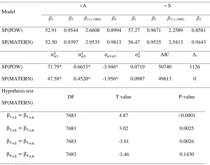
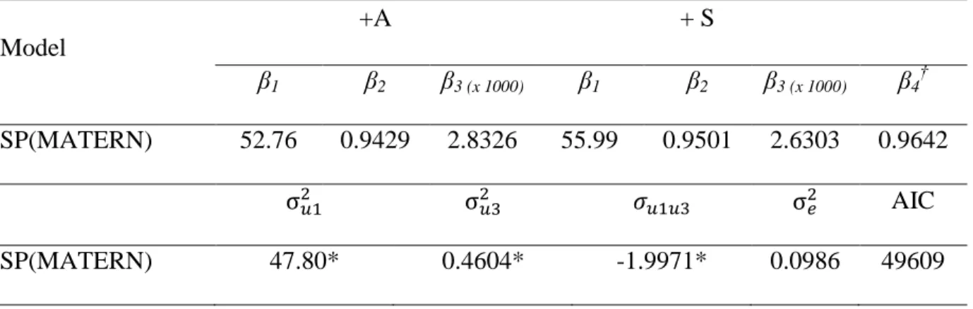
Using the SP(MATERN) error structure, there were differences between estimated parameters β1 (P < 0.0001), β2 (P = 0.0025), and β3 (P = 0.0026) of the genotypes evaluated; however, there was no difference in the β4 parameter (P = 0.1430) (Table 5). Therefore, the model was re-parameterized to account for just one β4 parameter. The final parameters adjusted for each genotype were as follows: β1 = 52.76 (SE = 0.463), β2 = 0.9439 (SE = 0.002), and β3 = 2.8326 (SE = 0.066) for the +A animals, and β1 = 55.99 (SE = 0.587), β2 = 0.9501 (SE = 0.002), and β3 = 2.6303 (SE = 0.079) for the +S animals. The common β4 parameter was 0.9642 (SE = 0.013). The variance components were 2u1 = 47.48, 2
u3 = 0.4604, and u1u3 = -1.9971 (P < 0.0001) (Table 6). The growth curves are shown in Figure 2.
The inflexion point was determined as a function of β4 (Richards, 1959). This parameter did not differ between the evaluated genotypes; the inflexion point at the same proportions of asymptotic body weight for both genotypes (36% of β1) yielded 19.05 kg and 20.22 kg for genotypes +A and +S, respectively.
18
and β4) in the functions, even when the errors were assumed to be independent. The variance power and error structure modeling yielded a better fit, and the Pearson residuals were within an acceptable range.
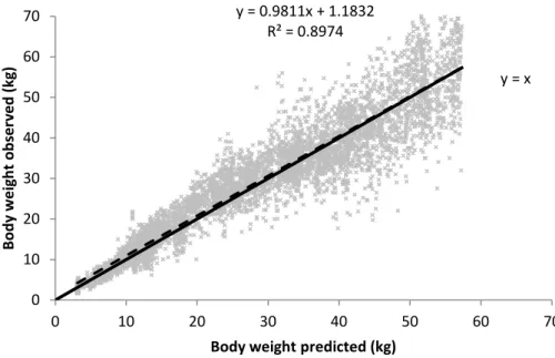
The Richards (u1 and u3) + VP + SP(MATERN) modeling approach was used to fit the training data set in the cross-validation analysis. The parameters estimated (data not show) did not differ from the parameters fitted from the original data set (P > 0.05), indicating that the chosen approach was effective even when using a reduced data set. When using the test data set to evaluate the model, the simultaneous F-test for the intercept (1.18 ± 0.14) and slope (0.98 ± 0.0045) rejected H0 (r² = 0.90). The CCC obtained was 0.95 (range from 0 to 1), indicating high accuracy. The RMSEP was 5.48 kg, and its decomposition indicated a high contribution from the random errors (98.37%), whereas the contributions of the mean bias (1.47%) and systematic bias (0.32%) were negligible. Figure 3 shows the relationship between the observed and predicted body weight values from the cross validation.
The Figure 4 shows that there was no apparent effect on the random parameter estimates from the number of weight measurements (Figure 4).
DISCUSSION
Growth curves and random effects
19
For models with only the variance component linked to asymptotic body weight, the error variation was partitioned into variation within goats ( ) and the variation between goats ( ). When two variance components were added to the variation between goats, the error variation was partitioned into variation due to asymptotic body weight, the sigmoidal-shaped curve of each animal, and the covariance between these terms (
and ) or due to the asymptotic body weight, rate constant, and covariance
between these terms ( and ), and so on, when 3 random effects were added; however, when three variance components were added in the growth curve model, there were indications of over-parameterization and more highly correlated parameters, causing problems with convergence and the hessian matrix.
In consequence, the estimate of the random effects (u1, u2, and u3) of each goat represents the deviation of a determined parameter from its corresponding parameter for its population average. For example, the mean asymptotic body weight of the population of goats with +A genotype is 52.7 kg (Table 6), and the specific estimate of random effects for a specific goat is 5.9 kg (empirical best linear unbiased prediction – EBLUP). Therefore, the mean asymptotic body weight estimated for this specific animal is 58.6 kg, independent of short-term fluctuations in weight due to extraneous environmental effects such as climate and food supply as well as lactation and pregnancy. Thus, the mean estimated parameters are not greatly affected by these types of weight fluctuations. In fact, these parameters represent the mean value of the growth pattern of the goats on the production system.
20
random effect estimate measures the difference between the value assigned to each individual and the average population value (Aggrey, 2009).
The high values observed for in most of the estimated models indicate the considerable contribution of this parameter in the residual variance component when this random variable is not added to the general model. Thus, it is important to incorporate this effect when using this methodology to estimate growth curves.
The component was almost always found to be significant. In addition, adding the random effects linked to the rate constant improved the estimated model fit, a fact that was validated by better selection criteria (residual variance and AIC) when including this component. Moreover, the significance of this parameter indicates that the rate constant varies among the goat population and is thus subject to breeding program selection.
A major advantage of selecting a nonlinear mixed model methodology to fit livestock growth curves is the possibility of including population variation measurements in stochastic models to predict animal performance. Normally, models predicting animal performance are deterministic, static, and empirical, and for the same input, there is only one output that is modeled from the averages, with little or no emphasis on population variation (Pomar et al., 2003). Therefore, when small samples are used, such as in the case of small farms, the errors become greater, especially when the model parameters vary greatly, as is the case for asymptotic body weight.
21
models, for which the biological principles are understood and explained, can make the predictions of such models more credible.
The significant differences in the asymptotic body weight and constant rate parameters of the data are indicative of differences in the growth pattern between the genotypes. Alpine goats likely achieve their mature weight earlier than do Saanen goats, as indicated by the higher rate constant of growth and lower asymptotic body weight estimated for this genotype. This knowledge can be used by farmers to choose between genotypes depending on their interest. Additionally, the different asymptotic body weights might be useful in mechanistic models, such as the Small Ruminant Nutrition Systems (SRNS) (Tedeschi et al., 2010), which makes use of this parameter in its set of equations to predict the degree of maturity for goats. This information is already available for cattle and some sheep genotypes; however, the data set pertaining to goats needs to be expanded.
The Von Bertalanffy, Logistic, and Gompertz models have a fixed inflection point (IP) relative to asymptotic body weight, which limits the biological interpretation of these functions due to the lack of flexibility in the estimation of the trend in the instantaneous absolute growth rate. In the case of the Richards model, the inflection point is variable and is a function of the β4 parameter. The best model had common parameter β4 = 0.9642 [IC95% 0.9394 – 0.9890], which yields a transitional function in form between the Brody (β4 = 0) and the Gompertz (β4 = 1) functions (Richards, 1959).
22
critical for plan optimization. Moreover, it is expected that from this point (~ 20 kg) onward, there is a decrease in growth rate, indicating a necessity for a change in feeding strategy.
Despite the fact that the genotypes have the same origin and are often considered similar in terms of productivity (only visibly different in their coats), differences have been found in their lactation curves (Guimarães et al., 2006), and now, in the present study, in their growth patterns. This result indicates the need to use separate models (growth, lactation, etc.) for these two genetic groups to predict animal response.
Modeling of the error structure
As noted by Littell et al. (2006), the first tool to be chosen when using the SAS software to fit a nonlinear mixed model is PROC NLMIXED, as it is more general because it accepts other distributions for the dependent variable; however, when it is necessary to model the error structure, the SAS macro %NLIMIX becomes more useful. Additional differences between the two approaches with relation to the estimation method can be found in Littell et al. (2006), Vonesh (2012).
23
The possible reason that the SP(MATERN) structure adjusted better to this data set is the difference between the measurements found here. Our data included between one and 1,190 days of difference between two consecutive measurements (lag). Obviously, two measurements taken at a close interval are typically more highly correlated than measurements taken at more distant time points (Littell et al., 2006). In our data set, 61% of the measurements were made before one year of life, which means that the data are temporally close; the inflection point calculated in the Richards models occurs at 19.05 kg and 20.22 kg for the +A and +S genotypes, respectively, which occurs at approximately 131 days of life. Measurements taken close to these points will be less correlated than measurements taken far from them due the higher instantaneous absolute growth rate observed around these inflection points. Figure 5 shows this relation.
Cross validation
Despite the fact that the simultaneous F-test for the intercept and slope rejected the null hypothesis, the high coefficient of determination indicates that the approach chosen is robust enough to estimate the body weight of goats. Furthermore, the RMSEP presented a relatively low value (5.48 kg) with a great contribution from random errors in the total error prediction. This finding indicates that effects that are not controlled are the main factors affecting the predictions. As shown in Figure 3, the predictions are more credible in the early phases of growth, at lower body weights; once there is a small variation around the average prediction, an increase in body weight leads to an occurrence of factors that are not controlled and operate to expand the variation around the estimated body weight; however, the average body weight estimated remains without bias, as indicated by the almost total overlap between the dashed line and the continuous lines.
24
The equations presented here are expected to yield more credible predictions for estimated mean values and population variations for some parameters.
Effects of number of weight values on the random effect estimates
Nonlinear mixed models are strong tools for modeling and understanding population variability by incorporating random effects to account for between-subject variations. Apparently, the lack of influence of the numbers of weight measurements on random effects is another advantage of this method. Thus, this approach can be used to select animals that are different from the population average with regard to their rate of growth and those with asymptotic body weight.
CONCLUSION
25
REFERENCES
Aggrey, S. E. 2009. Logistic nonlinear mixed effects model for estimating growth parameters. Poultry Science 88(2):276-280.
Beal, S. L. and L. B. Sheiner. 1982. Estimating Population Kinetics. CRC Crit. Rev. Biome. Eng. 8:195-222.
Brown, J. E., H. A. Fitzhugh, Jr., and T. C. Cartwright. 1976. A comparison of nonlinear models for describing weight-age relationships in cattle. J. Anim Sci. 42(4):810-818. Burnham, K. P. and D. R. Anderson. 2002. Model Selection and Multimodel Inference: A Practical Information-Theoretic Approach. 2nd ed. Springer-Verlag, New York.
Craig, B. A. and A. P. Schinckel. 2001. Nonlinear mixed effects models for swine growth. The Professional Animal Scientist 17:256-260.
Forni, S., M. Piles, A. Blasco, L. Varona, H. N. Oliveira, R. B. Lobo, and L. G. Albuquerque. 2009. Comparison of different nonlinear functions to describe Nelore cattle growth. Journal of Animal Science 87(2):496-506.
Guimarães, V. P., M. T. Rodrigues, J. L. R. Sarmento, and D. T. d. Rocha. 2006. Utilização de funções matemáticas no estudo da curva de lactação em caprinos. Revista Brasileira de Zootecnia 35:535-543.
Littell, R. C., G. A. Milliken, W. W. Stroup, R. D. Wolfinger, and O. Schabenberger. 2006. SAS for mixed models, second edition. Cary, NC: SAS Institute Inc.
Meng, S. X. and S. Huang. 2010. Incorporating correlated error structures into mixed forest growth models: prediction and inference implications. Canadian Journal of Forest Research 40(5):977-990.
26
Peek, M., E. Russek-Cohen, A. Wait, and I. Forseth. 2002. Physiological response curve analysis using nonlinear mixed models. Oecologia 132(2):175-180.
Pinheiro, J. C. and D. M. Bates. 1995. Approximations to the Log-Likelihood Function in the Nonlinear Mixed-Effects Model. Journal of Computational and Graphical Statistics 4(1):12-35.
Pinheiro, J. C. and D. M. Bates. 2000. Mixed-Effects Models in S and S-Plus. Springer, New York.
Pomar, C., I. Kyriazakis, G. C. Emmans, and P. W. Knap. 2003. Modeling stochasticity: Dealing with populations rather than individual pigs. J. Anim Sci. 81(14_suppl_2):E178-186.
Richards, F. J. 1959. A flexible growth function for empirical use. Journal of Experimental Botany 10(2):290-301.
SAS Institute Inc. 2008. SAS/STAT(r) 9.2 User's Guide. SAS Institute Inc., Cary, NC. Strathe, A. B., A. Danfaer, H. Sorensen, and E. Kebreab. 2010. A multilevel nonlinear mixed-effects approach to model growth in pigs. Journal of Animal Science 88(2):638-649.
Tedeschi, L. O. 2006. Assessment of the adequacy of mathematical models. Agricultural Systems 89:225-247.
Tedeschi, L. O., A. Cannas, and D. G. Fox. 2010. A nutrition mathematical model to account for dietary supply and requirements of energy and other nutrients for domesticated small ruminants: The development and evaluation of the Small Ruminant Nutrition System. Small Ruminant Research 89(2-3):174-184.
27
Vonesh, E. F. 2012. Generalized Linear and Nonlinear Models for Correlated Data: Theory and Applications Using SAS. SAS Institute Inc, Cary, NC, USA.
Wang, Z. and M. Zuidhof. 2004. Estimation of growth parameters using a nonlinear mixed Gompertz model. Poult. Sci. 83(6):847-852.
28 Table 1 – Summary of the data set assessed
Genotype nº of animals nº of weights
Max. obs. per goat
Min. obs. per goat
Max. age (days)
+S 498 4,292 21 4 2,666
+A 658 5,707 18 4 3,180
29 Table 2 – Evaluated growth curve functions
Model General function
Brody ̂ ( )
Von Bertalanffy ̂ (
Richards ̂ (
Logistic ̂ (
30
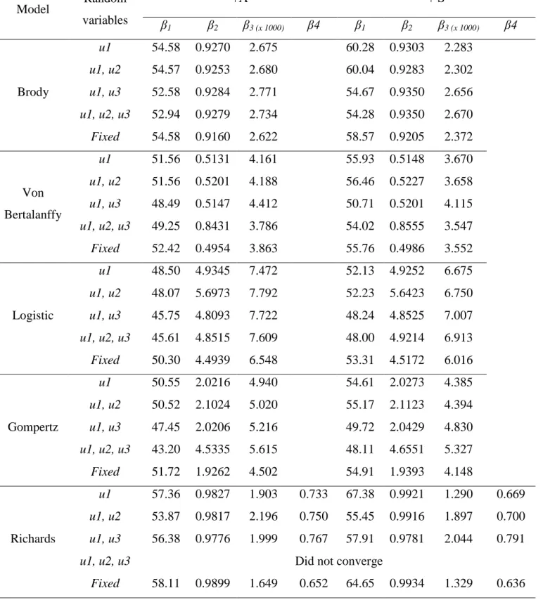
Table 3 – Estimated parameters for the different models, random variable combinations, and genotypes assessed
Model Random
variables
+A + S
β1 β2 β3 (x 1000) β4 β1 β2 β3 (x 1000) β4
Brody
u1 54.58 0.9270 2.675 60.28 0.9303 2.283
u1, u2 54.57 0.9253 2.680 60.04 0.9283 2.302 u1, u3 52.58 0.9284 2.771 54.67 0.9350 2.656 u1, u2, u3 52.94 0.9279 2.734 54.28 0.9350 2.670 Fixed 54.58 0.9160 2.622 58.57 0.9205 2.372
Von Bertalanffy
u1 51.56 0.5131 4.161 55.93 0.5148 3.670
u1, u2 51.56 0.5201 4.188 56.46 0.5227 3.658 u1, u3 48.49 0.5147 4.412 50.71 0.5201 4.115 u1, u2, u3 49.25 0.8431 3.786 54.02 0.8555 3.547 Fixed 52.42 0.4954 3.863 55.76 0.4986 3.552
Logistic
u1 48.50 4.9345 7.472 52.13 4.9252 6.675
u1, u2 48.07 5.6973 7.792 52.23 5.6423 6.750 u1, u3 45.75 4.8093 7.722 48.24 4.8525 7.007 u1, u2, u3 45.61 4.8515 7.609 48.00 4.9214 6.913 Fixed 50.30 4.4939 6.548 53.31 4.5172 6.016
Gompertz
u1 50.55 2.0216 4.940 54.61 2.0273 4.385
u1, u2 50.52 2.1024 5.020 55.17 2.1123 4.394 u1, u3 47.45 2.0206 5.216 49.72 2.0429 4.830 u1, u2, u3 43.20 4.5335 5.615 48.11 4.6551 5.327 Fixed 51.72 1.9262 4.502 54.91 1.9393 4.148
Richards
u1 57.36 0.9827 1.903 0.733 67.38 0.9921 1.290 0.669 u1, u2 53.87 0.9817 2.196 0.750 55.45 0.9916 1.897 0.700 u1, u3 56.38 0.9776 1.999 0.767 57.91 0.9781 2.044 0.791
u1, u2, u3 Did not converge
31
Table 4 – Variance and covariance components, residual variances, and information criteria of the fitted growth curves
Model Random
variables AIC Δr
Brody
u1 74.91* 12.92 57040 2354
u1, u2 80.01* 0.08* -4.0E-05ns 12.96 56999 2313
u1, u3 156.47* -13.29* 1.83* 8.66 54992 306
u1, u2, u3 160.53* 0.12* -13.19* -3.6E-04* -7.6E-03* 1.81* 8.82 54772 86
Fixed 33.46 63490 8804
Von
Bertalanffy
u1 64.77* 16.62 59293 4607
u1, u2 78.14* 0.17* 2.4E-03* 15.12 59083 4397
u1, u3 119.17* -16.87* 4.10* 10.79 57063 2377
u1, u2, u3 167.69* -6.68* -19.63* 0.73* 1.52* 3.91* 7.66 57287 2601
Fixed 37.69 64679 9993
Logistic
u1 56.26* 24.11 62627 7941
u1, u2 69.37* 8.53* 5.02* 19.94 62005 7319
u1, u3 93.07* -21.95* 9.72* 17.02 60983 6297
u1, u2, u3 106.51* 7.21* -20.62* 0.37** -1.87* 7.83* 16.72 60843 6157
Fixed 45.73 66613 11927
Gompertz
u1 61.78* 18.65 60323 5637
u1, u2 76.07* 1.12* 0.11* 16.32 59980 5294
u1, u3 110.08* -18.47* 5.43* 12.30 58207 3521
u1, u2, u3† 208.47 -99.11 -54.93 70.08 35.42 19.10 8.85 58134 3448
Fixed 39.88 65245 10559
Richards
u1 83.61* 11.91 56287 1601
u1, u2‡ 30.69 -1.0E-02 -1.7E-04 13.52 56900 2214
u1, u3 209.30* -13.01* 1.20* 8.50 54686 0
u1, u2, u3 Did not converge
Fixed 31.72 62960 8274
** - P<0.01; * - P<0.001 †
At least one eigenvalue was negative. ‡
Singular Hessian matrix.
ns–
32
Table 5 – Re-parameterized Richard model parameters with error structure
Model
+A + S
β1 β2 β3 (x 1000) β4 β1 β2 β3 (x 1000) β4
SP(POW) 52.91 0.9544 2.6608 0.8994 57.27 0.9671 2.2589 0.8581 SP(MATERN) 52.50 0.9397 2.9535 0.9813 56.47 0.9535 2.5413 0.9443
AIC Δr
SP(POW) 71.79* 0.6633* -3.946* 0.0719 50740 1126
SP(MATERN) 47.58* 0.4520* -1.956* 0.0987 49613 0
Hypothesis test SP(MATERN)
DF T value P-value
7683 4.87 <0.0001
7683 3.02 0.0025
7683 -3.01 0.0026
7683 -1.46 0.1430
33
Table 6 – Re-parameterized Richard model with error structure and just one β4 parameter
Model
+A + S
β1 β2 β3 (x 1000) β1 β2 β3 (x 1000) β4†
SP(MATERN) 52.76 0.9429 2.8326 55.99 0.9501 2.6303 0.9642
AIC
SP(MATERN) 47.80* 0.4604* -1.9971* 0.0986 49609
* P < 0.001
34
Figure 1 – Pearson residuals of the Richards functions versus predicted values (kg) using the following approaches: 1) Fixed-effects model; 2) random-effects model (u1 and u3); 3) random (u1 and u3) + VP + SP(MATERN).
-8 -4 0 4 8
0 20 40 60
P ear son r esi d u al s
Predict values (kg)
-8 -4 0 4 8
0 20 40 60
Predict values (kg)
-8 -4 0 4 8
0 20 40 60
Pear son r e si d u al s
Predict values (kg)
-8 -4 0 4 8
0 20 40 60
Predict values (kg)
-8 -4 0 4 8
0 20 40 60
Pear son r e si d u al s
Predict values (kg)
-8 -4 0 4 8
0 20 40 60
Predict values (kg)
1: +A 1: +S
2: +A 2: +S
35
Figure 2 – Adjusted growth curve for the two genotypes (+A, Alpine; +S Saanen) evaluated.
0 20 40 60 80 100
0 1000 2000 3000
B
o
d
y
w
eig
h
t
(k
g
)
Days
0 20 40 60 80 100
0 1000 2000 3000
Days
36
Figure 3 – Linear regression between observed and predicted body weights (dashed line). The continuous line is the Y = X line.
y = x y = 0.9811x + 1.1832
R² = 0.8974
0 10 20 30 40 50 60 70
0 10 20 30 40 50 60 70
B
o
d
y
we
ig
h
t
o
b
ser
v
e
d
(k
g
)
37
Figure 4 – Effect of the number of weight measurements on the random effects for the 1) u1 random parameter and 2) u3 random parameter.
-2.5 -1.5 -0.5 0.5 1.5 2.5
0 5 10 15 20
β1
ra
nd
o
m
ef
fec
t
Numbers of weighings -0.25
-0.15 -0.05 0.05 0.15 0.25
0 5 10 15 20
β3
ra
nd
o
m
ef
fec
t
Number of weighings
38
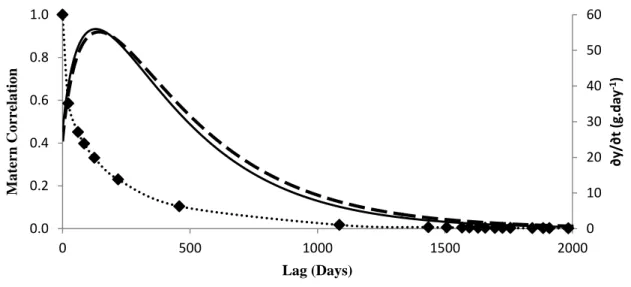
Figure 5 – The left axis shows the MATERN correlation function versus Lag (days) (point
line). Black diamonds (♦) correspond the values for animals with 21 weight measurements
during their lifetimes. The right axis shows the instantaneous absolute growth rate (g.day -1
) for +S animals (continuous line) and +A animals (dashed line).
0 10 20 30 40 50 60
0.0 0.2 0.4 0.6 0.8 1.0
0 500 1000 1500 2000
∂y
/∂
t
(g.
d
ay
-1)
M
a
ter
n
Co
rr
ela
tio
n
39
Running Head: Ruminal Fiber Stratification in Goats
Assessment of the heterogeneous rumen fiber pool and development of a mathematical approach for predicting the mean retention time of feeds in goats1
J. G. L. Regadas Filho*2; L. O. Tedeschi†; R. A. M. Vieira‡; M. T. Rodrigues*
* Departamento de Zootecnia, Universidade Federal de Viçosa, Viçosa, Minas Gerais 36570-000, Brazil.
† Department of Animal Science, Texas A&M University, College Station 77843-2471. ‡ Laboratório de Zootecnia e Nutrição Animal, Universidade Estadual do Norte
Fluminense Darcy Ribeiro (UENF), Campos dos Goytacazes, Rio de Janeiro 28013-602, Brazil.
1
The scholarship of the first author was supported by Coordenação de Aperfeiçoamento de Pessoal de Nível Superior – CAPES, Brazilian Government.
2
40 ABSTRACT
41
be assumed for goats fed diets with considerable fiber contents. The results of the sensitivity analysis indicated that both r and ke are of similar importance to the rate of passage in goats. The rates of passage of forage and concentrate in goats overlap and are closely related.
Key words: fractional rate of passage, Lucas’ test, sensitivity analysis, small ruminants.
INTRODUCTION
In applied ruminant nutritional models, the fiber pool has historically been assumed to be a compartment of uniform mass in the ruminoreticulum, regardless of the ruminant species considered. However, a uniform mass pool may not occur when animals are fed diets with considerable concentrations of fiber. Instead, in these cases, the digesta is stratified into two distinct solid phases, i.e., the floating mat (raft), which is selectively retained due to its buoyancy, and a solid phase containing smaller particles dispersed within the fluid phase that are able to escape from the rumen (Hungate, 1966, Sutherland, 1988, Vieira et al., 2008).
42
Our hypothesis is that goats, despite being considered browsers in natural environments (where the stratification of digesta would not occur), exhibit the non-selective behavior typical of roughage eaters when fed forage-based diets in confined and intensive production systems and therefore experience fiber pool stratification. Therefore, the objectives of this paper were to investigate the stratification of digesta in the rumen of goats, to develop a mathematical approach to predict the mean retention time of forage and concentrates in goats and to perform a sensitivity analysis of the models developed.
MATERIALS AND METHODS
Dataset Descriptions
The criteria used to select the studies to construct the database were those outlined by Cannas et al. (2003), in which diets must have at least 20% forage (DM basis); intake must have been individually measured, not estimated; rumen contents must have been measured by complete evacuation; and feed and rumen contents must have been analyzed for DM, CP, NDF, physically effective NDF (peNDF) and lignin. In addition, the pulse dose and fecal concentrations of the forage and concentrate markers had to be from the same animals that were used to measure the rumen content. The data from three studies were used as follows and summarized in Table 1.
43
Experiment 2 (Felisberto, 2011) evaluated the effect of the combination of three particle sizes (2, 5 and 15 cm (arithmetic mean particle size)) and four levels of NDF from forage (NDFf) (340, 410, 490 and 570 g∙kg-1 DM ) on the milk production of goats (after 60 days of lactation) in a 3 x 4 completely randomized factorial design. The data include 48 observations for rumen content collected 2 hours after feeding at slaughtering and profiles of fecal fiber excretion from forage and concentrates labeled with ytterbium and lanthanum, respectively.
Experiment 3 (Matos, 2012) studied the effect of three fiber sources (Tifton hay, corn silage and alfalfa hay) and number of parities (primiparous and multiparous) on the milk yield of dairy goats (after 60 days of lactation). This experiment consisted of a pen study with 96 dairy goats in 12 pens in a 3 x 2 completely randomized factorial design with two replicates. For each pen, two goats were slaughtered (2 hours after feeding) and three goats were used to measure the profiles of fecal fiber excretion. Thus, the average nutrients intake parameters, rumen content and particle kinetics were used. The data consisted of 12 values for nutrient intake, rumen content and profiles of fiber excretion from forage and concentrates labeled with ytterbium and lanthanum, respectively.
Testing for the Existence of a Single Fiber Pool
The validity of the single rumen fiber pool approach for goats was evaluated using the test developed by Lucas et al. (1961) and adapted by Van Soest et al. (1992) to identify homogenous compartments in the rumen. This approach has been used to predict the turnover of dietary components (Cannas et al., 2003) and the homogenous fiber compartment in cattle and sheep (Vieira et al., 2008). The uniform pool of a determined feed or digesta component in the ruminoreticulum compartment can only be considered if the linear relation between the pool size (Qx) and intake rate (Fx) yields acceptable
44
(1)
in which Qx and Fxare NDF or lignin rumen content and intake, expressed in g and g∙day -1
, respectively; Tx represents the ruminal turnover; and Qxm represents the metabolic portion of the component determined. The criteria adopted for the uniformity assumptions were the absence of a lack of fit for linear regression, a low value for the standard error of the linear regression parameters and an intercept that does not differ from zero for both NDF and lignin analysis, as fiber and lignin are not part of the endogenous matter (Van Soest, 1994). The uniformity assumption was tested by using all the data from Exp. 1 (n = 53), 2 (n = 48) and 3 (n = 12), because individual feed intake data were available and rumen contents were assessed by slaughtering all the animals.
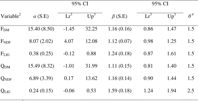
Additionally, the Qx and Fx were scaled to body weight using the allometric function . When β differed from unity (95% confidence interval), the scaled variables ⁄ and ⁄ were used to fit the linear regression (Eq. 1) and to evaluate the uniformity assumptions cited previously, yielding the variables and . If ; otherwise, , which contradicts the assumptions of fiber uniformity and indicates that the ruminal turnover is a function of
body weight, which is an additional assumption for applying the Lucas’ test (Vieira et al., 2008).
45
The Lucas’ test was performed using the following statistical model (Sauvant et al., 2008) via the MIXED procedure in the SAS software (SAS Inst. Inc., Cary, NC. version 9.3):
(2)
where Yij = the dependent variable (Qx or ), expressed in g; β0 = the overall (inter-study) intercept; Si = the random effect of the ith study, assumed to be independent and identically and normally distributed, or iid ~ N (0, σs2); β1 = the overall fixed regression coefficient of Y on X; Xij = the value of the continuous predictor variable (Fx or ), expressed in g∙day-1; bi = random effects of the regression coefficient of Y on X, assumed to be iid ~ N (0, b2); and eij = residual errors, assumed to be iid ~ N (0, σe2). When the SAS software produced the error message that the “estimated G matrix is not positive definite,” the model was re -parameterized without the respective variance component with a value of zero. Graphical analysis (conditional Pearson residuals vs. predicted values) indicated that there was within-subject (study) residual heteroscedasticity; thus, the power of the mean was used to account for this heteroscedasticity (Littell et al., 2006).
Rate Passage Analysis
The marker excretion profiles of the forage (Exp. 1 (n = 18), 2 (n = 48) and 3 (n = 12)) and concentrates (Exp. 2 (n = 48) and 3 (n = 12)) were kinetically interpreted with the model known as GNG1 (Eq. 3) (Matis, 1972, Matis et al., 1989, Pond et al., 1988, Vieira et al., 2008):
(
(
( { [ ( ] [ ( ] ∑ [ ( ] ⁄( }
46
in which δ = r/( r - ke); C(t) is the marker concentration at time ti; C(0) is the mass ratio between the marker dose and the particulate NDF mass of the raft pool; r is the age-dependent fractional rate for particle transference from the raft to the escapable pool (h-1); ke is the fractional rate of escape of particles from the escapable pool in the ruminoreticulum to the remaining parts of the stomach (h-1); is the particle transit time from the ruminoreticular orifice to the first appearance in the feces; and N is the order of time-dependency. The GNG1 model allows us to estimate the compartmental mean residence time (CMRT) independently for each ruminal pool (raft and escapable) and the mean retention time (MRT) can be expressed as ⁄ ⁄ , and the mean passage rate (kp) can be expressed as ⁄ .
The GNG1 functions were fitted to each profile for 0 < N ≤ 6 using the Marquardt algorithm of the NLIN procedure in SAS (SAS Inst. Inc., Cary, NC. version 9.3). The criteria adopted to choose the order of time-dependency were the following: 1) the convergence criterion; 2) estimates of r that did not tend towards ke; 3) the simplest model (smallest order of N), chosen using the approach described by Burnham and Anderson (2002) and Vieira et al. (2012) that used Akaike’s information criterion (AIC), differences among AIC values, the Akaike weights or likelihood probabilities and the evidence ratio or relative likelihood; and 4) graphical analysis.
Modeling Empirical Equations to Predict Ruminal Fractional Passage
47
other words, ⁄ ( . The second term was modeled directly in terms of the fractional rate ( .
The independent variable candidates that were common to all experiments were regressed against these parameters based on methods described by Tedeschi et al. (2012). Two groups of variables were used (Cannas et al., 2003): 1) predictors associated with diet composition, such as forage content (Fordiet), concentrate content (Concdiet), neutral detergent fiber (NDFdiet), crude protein (CPdiet) and lignin content (Ligdiet), which are expressed in g∙kg-1
DM; and 2) predictors associated with intake level, such as DMI, neutral detergent fiber intake (NDFI), intake of physically effective NDF (peNDFI, particles > 1.18 mm) and lignin intake (LIGI), which are expressed in g∙day-1. The
variables in group 2 were also expressed in g∙kg-1
BW (relative variables); however, when these parameters were determined to have body weight effects, the variables were scaled
to body weight (g∙kg-β
BW). In addition, the logarithms of all of the independent variables in group 2 were added. The logarithms of r and ke were also evaluated using the independent variables mentioned above (transformed variables). Because it has been shown that a relationship exists between the passage rates of concentrates and forage, the r and ke of forage and its logarithmic values were added to the r and ke of the concentrates as independent variables (Cannas and Van Soest, 2000).
48
(Tedeschi et al., 2012) to determine the combination of ⁄ and ke equations that best fit the dataset. Conditional Pearson residuals were used to evaluate the statistical assumptions and values outside the range of -3.0 to 3.0 were removed.
Sensitivity Analysis
A sensitivity analysis was performed using the Monte Carlo simulation technique to evaluate the impact of the independent variables on the dependent variable through the standardized regression coefficients (SRCs). The SRC reflects the change in the standard deviation of a dependent (output) variable associated with a unit change in the standard deviation of an independent (input) variable with all other variables held constant (Helton and Davis, 2002). The Monte Carlo simulation was performed with the @Risk v. 5.5.1 (Palisade Corporation, Ithaca, NY) software using 10,000 iterations and the default Latin hypercube sampling as the selection method. Certain biological aspects were considered by restricting the lower and upper limits of the independent variables in the probability distribution fitting. The predictors associated with intake (i.e., DMI, NDFI, etc.) were restricted as follows: ( ) . The predictors associated with diet composition (NDFdiet, LIGdiet, etc.) were restricted as follows:
( . The unknown bound specific to the distribution had a finite
bound (that is, it does not extend to plus or minus infinity). Spearman correlations were assigned to input variables to maintain the expected correlation between independent variables during the simulation. The Chi-squared statistic was used to choose the probability distribution for the independent variables.
RESULTS
49
assumption of the uniformity of the fiber pool. A value of β = 1 was used for the NDF intake and NDF rumen mass because neither parameter differed from unity. Consequently, the scaled variables were: ⁄ and ⁄ . For the lignin intake and lignin rumen mass, the following scaled variables were used: ⁄ and
⁄ .
The values of and did not differ from zero, which corroborates the homogeneous pool assumption. Furthermore, and were not different from each other (P = 0.84) (Table 3). Despite the lack of evidence of a difference between the power (P = 0.80) of the lignin intake and that of the lignin rumen mass (which would result in
and support the homogenous pool assumption), the intercept differed from
zero, indicating the presence of a potential metabolic component to the lignin, which is not possible (Table 3).
When the non-scaled variables were analyzed, there was clear heteroscedasticity of the residuals, indicated by θ values of 3.86 and 1.67 (P<0.001) for and , respectively, which suggests that MRT does not exhibit homogeneous behavior over the body weight range evaluated. The estimated variance components of the intercept and slope of the equations were not significant (P > 0.10) (Table 3).
50
Despite the low values of the approximate coefficients of determination of the above-mentioned equations, when the equations were formulated to predict the mean retention times, the R² and RMSE were 0.53 and 9.78 h, respectively, for forage and 0.49 and 5.86 h, respectively, for concentrates.
Table 5 shows the values of the Spearman correlation coefficients used to preserve the structure of the original dataset in the Monte Carlo simulation. The correlation coefficient values were maintained in the simulation even when they were not significant. It is interesting to note that the correlation coefficient value between ⁄ and was not significant (P = 0.20). However, a low but significant value for the correlation between ⁄ and (not shown in Table 5) was found (r = 0.39; P = 0.012).
Figure 2 shows the SRCs for the ⁄ and of forage (panels A1 and A2) and concentrates (panels B1 and B2) from the simulated predictions using the equations in Table 4. For the forage value of ⁄ , the NDFdiet and peNDFI are similar in intensity, but their effects have opposite signs; increasing the NDFdiet content also increases the time of residence in the raft pool, whereas increasing the peNDFI, decreases the residence time. For concentrates, increasing the DMI results in decrease in the residence time in the first fiber pool. Lignin intake has significant but opposite effects on the of forage and concentrates. It is interesting to note that LIGI has a strong influence on . An increase of one standard deviation in the LIGI value increases by 118%. Both concentrate pools were influenced by their respective forage pools. Figures 2-A3 and 2-B3 showed the effects of both fiber compartments on the rate of passage of fiber, calculated as
51
mean residence time (h), whereas the second pool was modeled in terms of the fractional rate (h-1).
Figure 3-A1 shows an overlap of the kp probability distributions for forage and concentrates. A pronounced overlap was observed between these probability distributions. In the simulated dataset, the mean with 99% confidence interval of the kp value for the forage was 0.0322 h-1 (0.0158 to 0.0556 h-1). For the concentrates, the mean kp value was 0.0334 h-1 (0.0146 to 0.0570 h-1), very close to the forage kp. Figure 3-B shows scatter plots of the simulated fractional rates of passage of forage and concentrates. A Pearson correlation coefficient of 0.66 (P< 0.001) was obtained.
DISCUSSION
Assessment of Heterogeneous Fiber Pools