On the modulation of the periodicity of the Faroe Bank Channel overflow instabilities

(1)

OSD

12, 823–861, 2015

FBC variability

E. Darelius et al.

Title Page

Abstract Introduction

Conclusions References

Tables Figures

◭ ◮

Back Close

Full Screen / Esc

Printer-friendly Version Interactive Discussion

Discussion

P

a

per

|

Discussion

P

a

per

|

Discussion

P

a

per

|

Discussion

P

a

per

|

Ocean Sci. Discuss., 12, 823–861, 2015 www.ocean-sci-discuss.net/12/823/2015/ doi:10.5194/osd-12-823-2015

This discussion paper is/has been under review for the journal Ocean Science (OS). Please refer to the corresponding final paper in OS if available.

On the modulation of the periodicity of the

Faroe Bank Channel overflow instabilities

E. Darelius1, I. Fer1, T. Rasmussen2, C. Guo1, and K. M. H. Larsen3

1

Geophysical Institute, University of Bergen and Bjerknes Centre for Climate Research, Bergen, Norway

2

Danish Meteorological Institute, Copenhagen, Denmark 3

Havstovan, Torshavn, Faroe Islands

Received: 7 April 2015 – Accepted: 30 April 2015 – Published: 21 May 2015

Correspondence to: E. Darelius ([email protected])

(2)

OSD

12, 823–861, 2015

FBC variability

E. Darelius et al.

Title Page

Tables Figures

◭ ◮

Back Close

Full Screen / Esc

Discussion

P

a

per

|

Discussion

P

a

per

|

Discussion

P

a

per

|

Discussion

P

a

per

|

Abstract

The Faroe Bank Channel (FBC) is one of the major pathways where dense, cold wa-ter formed in the Nordic Seas flows southward towards the north Atlantic. The plume region downstream of the FBC sill is characterized by high mesoscale variability, quasi-regular oscillations and intense mixing. Here, one year-long time series of velocity and 5

temperature from eight moorings deployed in May 2012 in the plume region is analyzed to describe variability in the strength and period of the oscillations. The eddy kinetic en-ergy (EKE) associated with the oscillations is modulated with a factor of ten during the year and the dominant period of the oscillations changes between three to four and six days, where the shorter period oscillations are more energetic. The dense water is 10

observed on a wider portion of the slope (both deeper and shallower) during periods with energetic, short period oscillations. The observations are complemented by results from a regional, high resolution model that shows a similar variability in EKE and a grad-ual change in oscillation period between three and four days. The observed variability in oscillation period is directly linked to changes in the volume transport across the sill: 15

the oscillation period decreases with about six days Sv−1_{both in the observations and}

in the model. This is in agreement with results from linear instability analysis which suggests that the period and growth rate decrease for decreased plume thickness. The changes in oscillation period can partly be explained by variability in the upper layer, background flow and advection of the oscillations past the stationary moorings, but 20

(3)

OSD

12, 823–861, 2015

FBC variability

E. Darelius et al.

Title Page

Tables Figures

◭ ◮

Back Close

Full Screen / Esc

Discussion

P

a

per

|

Discussion

P

a

per

|

Discussion

P

a

per

|

Discussion

P

a

per

|

1 Introduction

The Faroe Bank Channel (FBC) is the deepest connection between the Nordic Seas and the North Atlantic, and it carries an outflow of about 2 Sv (1 Sv≡106m3s−1) of cold, dense water formed north of the Greenland-Scotland ridge southwards (Hansen and Østerhus, 2007). Along its path, the overflowing water entrains and mixes with the 5

overlying, ambient water (Mauritzen et al., 2005; Fer et al., 2010) and makes a substan-tial – up to 25 % – contribution to the formation of North Atlantic Deep Water (Dickson and Brown, 1994).

Mooring records from the overflow plume region downstream of the FBC sill show energetic mesoscale variability; the dense water is observed to advance along the 10

slope in 100–200 m thick domes with a periodicity of 2–6 days (Darelius et al., 2011; Geyer et al., 2006). The domes are associated with a velocity signal extending through-out the water column and have a signature in the sea surface height (Darelius et al., 2013; Høyer and Quadfasel, 2001). Recent modeling eff_{orts suggest that the}

oscilla-tions are caused by growing baroclinic instabilities at the plume interface, manifested 15

as topographic Rossby waves in the upper layer (Guo et al., 2014).

Mesoscale oscillations are not uncommon on the continental slopes of the North At-lantic/Nordic Seas; Miller et al. (1996) report on barotropic oscillations with a period of 1.8 days further west (12◦W), on the southern side of the Iceland-Faroe Ridge, which they show to be wind-forced and linked to a resonant barotropic topographic Rossby 20

normal mode. Further north, Mysak and Schott (1977) describe fluctuations in the Nor-wegian current with a periodicity of 2–3 days that they find to be caused by baroclinic instabilities. Skagseth and Orvik (2002) show that variability in the same frequency range (and the same region) agree with topographic waves of the first mode, while slightly longer periods (3–5 days) correspond to the second mode.

25

(4)

OSD

12, 823–861, 2015

FBC variability

E. Darelius et al.

Title Page

Tables Figures

◭ ◮

Back Close

Full Screen / Esc

Discussion

P

a

per

|

Discussion

P

a

per

|

Discussion

P

a

per

|

Discussion

P

a

per

|

et al., 2009). The eddies modify vertical mixing and entrainment (Darelius et al., 2013), induce horizontal stirring (Voet and Quadfasel, 2010; Darelius et al., 2013) and influ-ence the descent rate of the dense water (Seim et al., 2010). The intensity of eddy generation will thus aff_{ect the final properties and pathway of the overflow end product,}

the North Atlantic Deep Water. 5

Based on the first one year-long mooring record from the plume region (Ullgren et al., 2015), the modulation of the strength and in the dominant time scale of the mesoscale variability is described, and found to be substantially modulated throughout the year. The modulation of the oscillations and its coupling to oceanic and atmospheric forcing are explored and the analysis is extended to include results from a high resolution 10

regional model (Rasmussen et al., 2014).

2 Data and methods

2.1 Moorings, 2012/13

Data were collected in the Faroe Bank Channel overflow region using eight bottom-anchored moorings in the period from 28 May 2012 to 5 June 2013 (Fig. 1). Three 15

of the moorings were deployed in the channel (the C array), and five on the open slope about 80 km downstream of the sill (the S array and mooring M1). The moorings were equipped with temperature, conductivity and pressure recorders in addition to current meters. Further information on the moorings can be found in Ullgren et al. (2015) and in Table 1. The coordinate system for each mooring is aligned with the 20

orientation of the corresponding mooring array, so that thex axis is perpendicular to the array and the y axis parallel to the array, pointing upslope. The angle of rotation is 34 and 31◦ (clockwise) for the C and S array respectively. Hourly mean data are interpolated to a grid with 1 m vertical resolution following the procedure outlined in Darelius et al. (2011). Velocity data from periods when the instrument tilt exceeds the 25

(5)

OSD

12, 823–861, 2015

FBC variability

E. Darelius et al.

Title Page

Tables Figures

◭ ◮

Back Close

Full Screen / Esc

Discussion

P

a

per

|

Discussion

P

a

per

|

Discussion

P

a

per

|

Discussion

P

a

per

|

causes a slight bias towards lower velocities (since drag, and thus tilt, is larger for increasing velocities). The percentage of data discarded for any instrument is less than 3 %.

When the focus is on the evolution of the background field and not on the oscillations, the hourly data are filtered using a low-pass Butterworth filter of 4th order. The cut-off

5

frequency is 30 days unless otherwise stated in the text where filtered data is discussed or shown.

Wavelet analysis is used to identify the dominant periods of variability and to describe how these change in time. The analysis is carried out using the hourly data and a Morlet mother function, and the 95 % significance level is found using a regular chi-square test 10

(Torrence and Compo, 1997). The dominant oscillation period is defined as the period with highest, significant energy level at each time step.

The eddy kinetic energy (EKE) associated with the oscillations is estimated by inte-gration using

EKE=

f2 Z

f₁

(Θ_u+ Θ_v_{) d}_f_, ₍₁₎

15

wheref₁=₁_/_{6 cycles per day (cpd),}_f

2=2/5 cpd, andΘu/v is the power spectral den-sity in the along/across slope direction respectively. The presented EKE values are vertical means over the depth range with velocity measurements, see Table 1, ex-cept for S3 where only data from the upper Acoustic Doppler Current Profiler (ADCP), i.e. above the plume, are used. The EKE is normalized with the maximum value in 20

respective time series. The EKE values are artificially elevated at the plume interface, since an instrument at a given level there is located alternatively in and out of the plume (see Ullgren et al., 2015). While it would be of interest to compare absolute EKE values from levels not aff_{ected by the plume, such are available only from S3. Time series of}

EKE is obtained by first calculatingΘ

(6)

OSD

12, 823–861, 2015

FBC variability

E. Darelius et al.

Title Page

Tables Figures

◭ ◮

Back Close

Full Screen / Esc

Discussion

P

a

per

|

Discussion

P

a

per

|

Discussion

P

a

per

|

Discussion

P

a

per

|

Θ

v separately gives EKEv, i.e. the EKE associated with motion in the across slope direction.

The transport,Q_T, of water colder thanT◦_{C past a mooring array is estimated from}

Q_T(t)=

n X

i=₁

ziZ,T(t)

0

u_i(z,t)L_idz, (2)

where n is the number of moorings in the array, ui is the velocity perpendicular to 5

the array at mooring i, z_i_,_T the height of theT ◦_{C isotherm at mooring} _i_{, and} _L

i the representative width of the mooring. The distance between C1 and C2 is 7 km and the distance between C2 and C3 is 8 km andL is taken to be 7, 7.5 and 8 km for C1, C2 and C3, respectively. The transport values given are calculated usingT =₆◦_{C, which}

roughly corresponds to σθ=27.7 kg m−3 and density range 3–5 in Mauritzen et al. 10

(2005).

2.2 FBC-sill moorings

The mooring records from the plume region in 2012/13 described above are comple-mented with data from the long-term monitoring mooring from the FBC sill (Hansen and Østerhus, 2007). Moorings have been deployed quasi-continuously from 1995 un-15

til present at the location FB on the FBC sill (see Fig. 1 for location). Contemporary measurements from the sill (FB) and the plume region exist during the period June 2012–June 2013, when an upward looking ADCP (RD-Instruments 75 kHz BroadBand) was deployed at FB.

The data from FB consist of velocity profiles only, with no explicit information about 20

(7)

OSD

12, 823–861, 2015

FBC variability

E. Darelius et al.

Title Page

Tables Figures

◭ ◮

Back Close

Full Screen / Esc

Discussion

P

a

per

|

Discussion

P

a

per

|

Discussion

P

a

per

|

Discussion

P

a

per

|

2.3 Other data sets

Meteorological data (wind, pressure and temperature) from DMI are available from a weather station in Torshavn, Faroe Islands (Cappelen, 2014) with a temporal reso-lution of 3 h. Daily, gridded fields of sea level height anomalies (SLA) and geostrophic velocity anomalies calculated from satellite altimetry for the period and region of inter-5

est have been downloaded from http://www.aviso.altimetry.fr.

2.4 Numerical model

The model is a slightly modified version of the HYbrid Coordinate Ocean Model (HY-COM) v2.2.18 (Bleck, 2002; Chassignet et al., 2007). HYCOM exploits a hybrid coor-dinate system that is isopycnal in the open, stratified ocean, but smoothly reverts to 10

a terrain-following coordinate in shallow coastal regions, and toz level coordinates in the mixed layer and/or unstratified seas. The vertical mixing is defined by the K-profile parameterization (KPP-scheme; Large et al., 1994). The horizontal grid size ranges from 750 to 1300 m and the resolution is highest near the Faroe Islands. This model setup has 32 vertical layers, 340 grid points in the southwest/northeast direction and 15

400 grid points in the southeast/northwest direction. The model domain is shown in Fig. 1. The bathymetry is extracted from ETOPO1 (Amante and Eakins, 2009) com-bined with measurements conducted by the Faroe Marine Research Institute (FAMRI) and the coast guard (Simonsen et al., 2002).

The barotropic velocities are prescribed on the boundary along with the sea sur-20

face height, whereas the baroclinic velocities, the temperature and the salinity are prescribed by a relaxation towards the boundary conditions (provided by a hindcast archive from the Danish Meterological Institut covering the Arctic and the North Atlantic Ocean) on the outermost 10 grid points. The time scale of relaxation on the boundary is one day, and decreases linearly to 10 days on the 10th grid point from the boundary. 25

(8)

OSD

12, 823–861, 2015

FBC variability

E. Darelius et al.

Title Page

Tables Figures

◭ ◮

Back Close

Full Screen / Esc

Discussion

P

a

per

|

Discussion

P

a

per

|

Discussion

P

a

per

|

Discussion

P

a

per

|

stress and the atmospheric vapor mixing ratio. The forcing is prescribed with a tem-poral resolution of 3 h and a spatial resolution of 79 km, which is interpolated to the model grid. Further details can be found in Rasmussen et al. (2014). In addition to the model output fields, time series for detailed analysis is extracted from a virtual mooring “M” on the slope (see Fig. 1).

5

3 Results

3.1 The FBC overflow plume

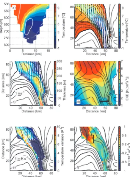
The FBC, located between the Faroe Plateau (FP) in the north and the Faroe Bank (FB) in the south, is about 840 m deep and less than 15 km wide at the sill. Results from the numerical model (Fig. 2) are used to illustrate the description of the FBC over-10

flow plume. In the channel, the outflow forms a 200 m thick, cold layer leaning on the FP, with core velocities on the order of 1 m s−1 _{(Fig. 2a, e.g. Hansen and Østerhus,}

2007; Hansen et al., 2001). The cold water continues to flow northwestward along the slope as a dense, gravity-driven plume that widens and thins as the channel opens up (Fig. 2b; Mauritzen et al., 2005). Downstream of the sill, baroclinic instabilities de-15

velop (Guo et al., 2014) and the dense plume breaks up into domes of cold water that are associated with eddies in the upper layer (Fig. 2c and d, Darelius et al., 2013). Following the procedure outlined in Bishop et al. (2013) and Guo et al. (2014), the divergent eddy heatflux (EHF) and the associated baroclinic conversion (BC) rate are calculated using one month long subsets of the HYCOM model results. Figure 2e and 20

f show examples of EHF and BC-fields from August 2008, interpolated to 100 m above bottom (mab, fields are calculated in horizontal layers every 10th m in the vertical). The results are similar to those shown by Guo et al. (2014), with upslope divergent eddy heat fluxes and high baroclinic conversion rates (BC≈10−5m2s−3) appearing about 40–60 km downstream of the sill at the deeper edge of the dense plume.

(9)

OSD

12, 823–861, 2015

FBC variability

E. Darelius et al.

Title Page

Tables Figures

◭ ◮

Back Close

Full Screen / Esc

Discussion

P

a

per

|

Discussion

P

a

per

|

Discussion

P

a

per

|

Discussion

P

a

per

|

3.2 Temporal evolution of mesoscale variability on the slope

The mooring records from the slope array show energetic oscillations in temperature and velocity with a period varying between 3 and 6 days (Fig. 3), similar to those described in Geyer et al. (2006); Darelius et al. (2011, 2013). While Geyer et al. (2006) stated that the oscillations were “highly regular”, the present, longer observation 5

records show that the intensity and the periodicity of the oscillations vary considerably in time. A direct inspection of the velocity records and wavelet analysis (Fig. 3d) sug-gests that the periods of oscillations alternate between three-four days and six days, where the low amplitude (i.e. less energetic) oscillations typically have longer periods. Based on the oscillation characteristics, the time series has been divided into six in-10

tervals, T1–6 (see Table 2–3 and Fig. 3). In all mooring locations, the EKE associated with the oscillations shows high values in August, January–February and in April, and a minimum in early winter (October–December, Fig. 3e). The intra-seasonal variability is large, e.g. at S3 the November EKE is only 10 % of the maximum value.

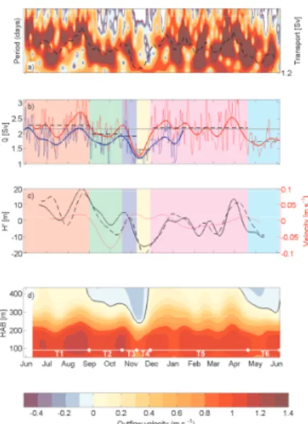
In the numerical model, the dominant periodicity of the oscillations is 3–4 days 15

(Fig. 4a–d), similar to the observations. Unfortunately, a direct comparison is not possi-ble because the model was not run for a period overlapping with the observations. The variability of the oscillations in the model, nevertheless, shows similarities with that in the observations: the EKE associated with the oscillations on the slope (at mooring M) varies by a factor of ten, with a minimum in March–April and a maximum in August– 20

September (Fig. 4e). A comparison of Fig. 3d (observations) and Fig. 4d (model), how-ever, shows that while the oscillations in the observations alternate between shorter (3–4 days) and longer (6 days) period, the change in period of the model oscillations is relatively gradual and appears to follow a seasonal cycle; it decreases from about four days in summer to about three days in November–December and then increases again 25

(10)

OSD

12, 823–861, 2015

FBC variability

E. Darelius et al.

Title Page

Tables Figures

◭ ◮

Back Close

Full Screen / Esc

Discussion

P

a

per

|

Discussion

P

a

per

|

Discussion

P

a

per

|

Discussion

P

a

per

|

Figure 2f shows the baroclinic conversion (BC) rate associated with the oscillations in the numerical model. Time series of BC are constructed using the monthly mean value in an area (see Fig. 2) about 40–60 km downstream of the sill. The BC shows a maximum in August, and two minima: November and March (Fig. 4f). The time series of BC closely follows the EKE at M (Fig. 4e).

5

3.3 Modulation by the overflow at the sill

Time series of kinematic overflow measured at FB are shown in Fig. 5b together with the volume flux of water colder thanT =₆◦_{C past array C (see Sect. 2.1 for calculation}

details). During the period with overlapping measurements, the low passed transport time series from FB and array C correlate well with a correlation coeffi_{cient of 0.9. The}

10

transport estimates from array C are lower by a factor of 0.84 compared with the kine-matic overflow at FB. As discussed in e.g. Hansen and Østerhus (2007), the transport across the sill shows considerable variability on both daily and monthly time-scales. A relationship between the low passed (14 days) transport across the sill and the dom-inant period of the oscillations on the slope is apparent in Fig. 5a and further quantified 15

in Fig. 6. Here, at each time step the dominant oscillation period (i.e. the oscillation period with the highest, significant energy level) from the wavelet analysis (shown in Figs. 3d and 5a) and the transport have been identified, and the transport is averaged in bins of oscillation period. Times of high transport coincide with shorter oscillation periods and times with low transport with longer oscillation periods. Linear regression 20

gives a decrease in oscillation period of about 5.8 days Sv−1_{for the observations.}

The modeled transportQ across the sill displays a seasonal signal, increasing from 1 Sv in summer to 1.5 Sv in autumn (Fig. 4g). The observations from 2012/13 do not show a seasonal signal in transport, although a seasonality (of about the same ampli-tude but shifted in time with respect to the numerical model) emerges when combining 25

(11)

OSD

12, 823–861, 2015

FBC variability

E. Darelius et al.

Title Page

Tables Figures

◭ ◮

Back Close

Full Screen / Esc

Discussion

P

a

per

|

Discussion

P

a

per

|

Discussion

P

a

per

|

Discussion

P

a

per

|

are approximately 1 Sv lower than the observations. Note that longer period oscillations are only found during one short interval in the modeled time series.

The mean plume thickness, H, here defined as the height of the 6◦C isotherm, in the core of the plume on the slope (S2 and S3) shows variability (Fig. 3c) similar to the transport estimated from the mooring arrays in the channel (C and FB, Fig. 3b). The 5

plume thickness recorded at S2 and S3 are typically in phase, implying that the variabil-ity is not caused by plume meandering. During periods with more intense oscillations and higher than normal plume thickness at S2 and S3 (T1 and T5), cold plume water is more often than normal present at the upper (S1) and lower (S4) mooring in the array (see Table 3). During T4, temperatures recorded by these moorings were above 3◦C 10

at all times. A time series of monthly mean plume thickness (from the box marked in Fig. 2f) in the numerical model is shown in Fig. 4f. The mean plume thickness mimics the curves of EKE (Fig. 4e) and BC (Fig. 4f).

3.4 Currents in the upper layer

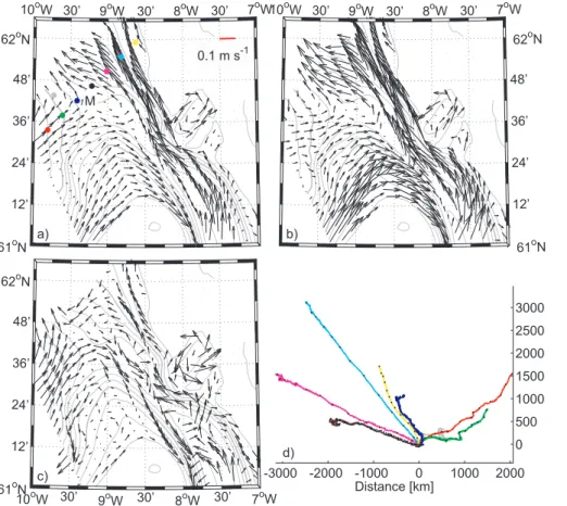
The modeled upper layer velocities (300 m depth) are shown in Fig. 7. Atlantic origin 15

water flows northwestward along the Iceland-Faroe slope on the Faroe Plateau side. The current is stronger and extends further out from the shelf in August than in March. Meanwhile, there is a clockwise circulation around the Faroe Bank, causing a relatively strong shear across the FBC (a similar shear is observed in mooring data from the sill; Hansen and Østerhus, 2007). This current is also stronger in August than in March, 20

when it has shifted westward following deeper isobaths and therefore to a lesser extent enters the FBC. In the model, most of the water entering the Faroe Shetland Channel through the FBC recirculates and returns northwestward with the current on the Faroe Plateau side. In the numerical model, a seasonal signal similar to that observed in the transport across the sill and in the periodicity of the observations is apparent in the 25

(12)

OSD

12, 823–861, 2015

FBC variability

E. Darelius et al.

Title Page

Tables Figures

◭ ◮

Back Close

Full Screen / Esc

Discussion

P

a

per

|

Discussion

P

a

per

|

Discussion

P

a

per

|

Discussion

P

a

per

|

The changing characteristics of the observed oscillations coincide with the variabil-ity in the upper layer circulation. The observed vertical mean current between 150 and 500 m depth (i.e. well above the plume; Ullgren et al., 2015) at S3 is shown in Fig. 8a as progressive vector diagram and in Fig. 8b as vectors giving the mean velocity during T1–6. Above the plume, the velocity profiles show little variability in the vertical, sug-5

gesting a barotropically-forced current. The direction of theu_up changes dramatically from northeastward in T1 to southeastward in T2 and northward in T3. During intervals T2, T4 and T6 the mean upper layer current has a component directed towards the sill (i.e. opposing the dense overflow). The intervals with sill-ward flow are associated with anomalous inflow at the sill at depths shallower than 250–350 mab, and relatively 10

weak outflow at FB (Fig. 5d). Geostrophic velocity anomalies calculated from satellite altimetry for the period and the region of interest are shown in Fig. 8c–h. Geostrophic current anomalies during T2, T4 and T6 are directed towards the sill, in fair agreement with the observations from S3 and FB.

There is no significant correlation between the along slope current in the upper layer 15

at S3 and the transport across the sill, but upon inspection of Figs. 3, 5 and 8, a pattern emerges whereby low amplitude, long period or irregular oscillations occur when the mean upper layer current is sill-ward while energetic, relatively regular and shorter period oscillations occur when the mean upper layer current is transverse to the dense overflow. The properties of the oscillations and the plume during T1–6 are summarized 20

in Table 3.

3.5 Barotropic forcing of the FBC outflow

The results presented in Sect. 3.4 suggest a relationship between the overflow trans-port variability and the local barotropic forcing on intra-seasonal time scales. The sea-sonal variability in the transport of dense water through the FBC has previously been 25

(13)

er-OSD

12, 823–861, 2015

FBC variability

E. Darelius et al.

Title Page

Tables Figures

◭ ◮

Back Close

Full Screen / Esc

Discussion

P

a

per

|

Discussion

P

a

per

|

Discussion

P

a

per

|

Discussion

P

a

per

|

ence∆_{SLA correlates with a correlation coe}ffi_{cient greater than 0.65 with the transport}

across the FBC sill (all possible combinations of grid points within the area shown have been tested). High transport values coincide with high SLA on the Faroe Plateau and low SLA above the slope, i.e. with a geostrophically balanced barotropic current aligned with the slope and the dense outflow. The time series of ∆_{SLA between the}

5

combination of grid points giving the highest correlation with the transport is shown in Fig. 9b. A correlation of 0.71 indicates that about 50 % of the variance can be explained by the local barotropic forcing. Variability in∆_{SLA with typical amplitudes of 0.1 m and}

time scales of 2–4 weeks coincides with the variability in transport, which has an am-plitude of about 0.5 Sv. Linear regression gives ∆_Q=_k∆_{SLA where} _k=_{6.5 Sv m}−1_.

10

A sea level diff_{erence of 0.1 m between these two points, located 145 km a part, would}

give a mean barotropic current of about 0.05 m s−1, roughly corresponding to a change in transport across the sill on the order of 0.15 Sv (assuming a cross sectional area for the outflow of about 15 km×200 m). The sensitivity obtained from the linear regression of∆_{SLA against}_Q _{is four times higher (an increase in}∆_{SLA of 0.1 m corresponds to}

15

an increase inQof 0.65 Sv) suggesting that the barotropic current is more focused and thus stronger in the sill region than above the Iceland-Faroe slope. Indeed, the agree-ment in sensitivity between∆_{SLA and}_Q_{for points located more directly across the sill}

is better (with a factor of two). Note that with the kinematic definition of plume thickness used in the estimate ofQ from FB, a barotropic current would not only influence the 20

outflow velocity, but also the plume thickness. For the mean velocity profile from FB, the increase in kinematic interface height caused by a barotropic current of 0.1 ms−1is 6 m, or approximately 3 % of the typical plume thickness.

4 Discussion

Recent results from a semi-idealized numerical model suggest that the eddies or os-25

(14)

OSD

12, 823–861, 2015

FBC variability

E. Darelius et al.

Title Page

Tables Figures

◭ ◮

Back Close

Full Screen / Esc

Discussion

P

a

per

|

Discussion

P

a

per

|

Discussion

P

a

per

|

Discussion

P

a

per

|

a parabolic shaped plume on a sloping bottom using the model developed by Reszka et al. (2002) and parameters relevant for the FBC overflow (Guo et al., 2014) yields that the period and wavelength of the most unstable wave decrease and the growth rate in-crease with increasing plume thickness (Fig. 10a). These results are in agreement with the observations presented in Sect. 3. The oscillation period decreases for increasing 5

transport across the sill and a thicker plume and, while there are exceptions, the EKE tends to be high when the plume is thick and the volume transport is large (e.g. August and April), and low when the plume is thin and the volume flux is low (e.g. November). The link between the plume thickness, BC and EKE is even more obvious in the realisti-cally forced numerical model, and the same tendency was observed in the experiments 10

of Guo et al. (2014). The dominant period and the transport across the sill are obtained for the five sensitivity runs discussed in Guo et al. (2014) and the results are included in Fig. 6. Note that the forcing – and thus the transport and also the oscillation pe-riod is quasi-constant for each of the runs. The sensitivity in the oscillation pepe-riod to changes in transport in these, highly idealized model runs (forced solely by a dense in-15

flow through the FSC on the northern boundary) is much smaller (₋0.6 days Sv−1_{) than} in the observations and in the more realistic model setup described in this paper. Why is the oscillation period in the idealized model runs much less sensitive to the overflow transport than the observations and the realistic modeling? One possible reason is, that while the transport variability in the observations and in the realistic model to a large 20

extent is caused by barotropic forcing (see Fig. 9) the increased flux in the idealized model is due solely to increased baroclinic forcing. In addition, the observations and the realistic model show a barotropic velocity shear (Fig. 7) in the sill region that pos-sibly modifies the disturbances generated by the baroclinic instability (Pedlosky, 1986, p. 582–589).

25

(15)

mod-OSD

12, 823–861, 2015

FBC variability

E. Darelius et al.

Title Page

Tables Figures

◭ ◮

Back Close

Full Screen / Esc

Discussion

P

a

per

|

Discussion

P

a

per

|

Discussion

P

a

per

|

Discussion

P

a

per

|

ulates the flow and the transport across the sill. A barotropically forced background current aligned with the outflow across the sill increases the transport of dense water, but neither the plume thickness nor the baroclinic shear through which the baroclinic instabilities grow would be aff_{ected locally. Further downstream, however, where the}

barotropic forcing disappears or weakens (e.g. as the barotropic current follows the 5

shelf break to the northwest) the plume thickness and/or the baroclinic shear must be altered in order to maintain the increased transport of dense water along the slope. Thus, we expect an increased barotropic forcing at the sill to alter the conditions for baroclinic instability downstream and hence the intrinsic period of the most unstable wave. At the same time, a barotropically forced flow aligned with the plume path will 10

influence the periodobservedat a stationary mooring, sinceT_obs=_λ/₍_c+_v_{), where}_λ_is

the wavelength,cthe phase velocity andv component of the background (barotropic) current that is aligned with the phase velocity. T_obs decreases if the mean flow is in the direction of the phase speed of the wave and increase if the current is oppositely directed (see Fig. 10c). Throughout the year, the modeled upper layer velocity in the 15

along-slope direction at M increases from nil tou_up=_{0.1 m s}−1_{(Fig. 4f) and for a}

typi-cal wavelength-wave number pair obtained from the instability analysis (Reszka et al., 2002; Guo et al., 2014) the corresponding reduction in the observed periodicity would be about 1 day (Fig. 10c), possibly explaining most of the variability in the period in the model results (Fig. 4d).

20

The results by Reszka et al. (2002) suggest that baroclinic instabilities appear as an amplifying topographic Rossby wave (TRW) in the upper layer of a two-layer flow with a continuously stratified upper layer. The observations described in Darelius et al. (2011) and Darelius et al. (2013) are consistent with TRWs. For such waves, and for the parameters relevant in the FBC (Darelius et al., 2011), the dispersion relation is 25

given byω=_sN_sin_α_{, where}_s=_{0.01 is the slope,}_N=₃_×₁₀−3_s−1_{the average}

(16)

OSD

12, 823–861, 2015

FBC variability

E. Darelius et al.

Title Page

Tables Figures

◭ ◮

Back Close

Full Screen / Esc

Discussion

P

a

per

|

Discussion

P

a

per

|

Discussion

P

a

per

|

Discussion

P

a

per

|

velocity is caused by the wave motion. According to the dispersion relation, the trans-verse motions of the waves changes from along-slope orientation for low-frequency waves to increasingly cross-slope orientation at higher frequencies (Pickart and Watts, 1990). We would thus expect the fraction of the EKE in the cross slope component,

β_v=_EKE

v/EKE, to decrease during time periods with a longer oscillation period, and 5

increase with a shorter oscillation period. Time series of βv is calculated from levels above the plume at S3 and shown in Fig. 11. Consistent with theory, there is a tendency for low values ofβ_v during time periods with longer oscillations, e.g. in November and May. This suggest that the variability in the observed oscillation period is (at least partly) due to changes in the intrinsic period and not (only) to variable upper layer velocities 10

and advection.

The regular oscillations observed by Geyer et al. (2006) change character towards the end of their measurement period; in October the period increases from 88 h to more than 5 days and towards the very end of the record the oscillations seemingly disap-pear (see their Fig. 9). The disapdisap-pearance coincides with a relatively strong geostrophic 15

velocity anomaly directed towards the sill (not shown). In a similar manner, the oscil-lations on the slope change character in the beginning of June 2008, as discussed by Darelius et al. (2011). This occurs when the geostrophic velocity anomaly (inferred from AVISO) changes from being mainly aligned with the dense outflow (Fig. 12a) to a situation with relatively strong southeastward flow above the lower part of the slope 20

(Fig. 12b). It was shown that the changing oscillations on the slope in 2012/13 were associated with inflow anomalies above the outflow at the sill (Fig. 5d), similar (but weaker) anomalies are observed at FB in October and November 1999 and in June 2008 (when the oscillations in respectively Geyer et al., 2006 and Darelius et al., 2011 change character).

25

(17)

OSD

12, 823–861, 2015

FBC variability

E. Darelius et al.

Title Page

Tables Figures

◭ ◮

Back Close

Full Screen / Esc

Discussion

P

a

per

|

Discussion

P

a

per

|

Discussion

P

a

per

|

Discussion

P

a

per

|

more regular oscillations in the numerical model compared to the observations (i.e. the smoothness of Fig. 4d compared with Fig. 3d). The brief increase in oscillation period in the modeled time series during March 2009, coincides with a weak (relative to the observations) inflow event.

The baroclinic instabilities grow fastest once the dense water exits the channel onto 5

the open slope (high BC values in Fig. 2). The oscillations, however, are present al-ready at the sill; Saunders (1990) describes observation of oscillations with a period of 3–6 days in the sill region and the EKE in the numerical model show elevated val-ues on the FB side of the sill (Fig. 2d). Model results by Guo et al. (2014, see their Fig. 3) and Seim et al. (2010) show fluctuations in plume transport also at the sill. 10

During the period with concurrent measurements at FB and the slope, the EKE at the sill broadly follows that on the slope (Fig. 3), although energy levels are much lower (the annual mean is about 100 cm2s−2 in the upper layer compared to 300 cm2s−2 at S3, not shown). The dense outflow across the FBC-sill shows a maximum during the summer months (June–September) and a minimum during winter (December–March, 15

Hansen and Østerhus, 2007, their Fig. 23) that is linked to the seasonality in the inflow of Atlantic water towards the Nordic Seas through the FSC; the barotropically forced northeastward flow modulates the southwestward flow of dense waters at depth which is feeding the FBC overflow (Lake and Lundberg, 2006). The thickness of the outflow across the sill (defined as the level where the velocity is 50 % of the maximum velocity) 20

shows a similar seasonal variability (Hansen and Østerhus, 2007) and following the results from Reszka et al. (2002), we would expect the EKE to show the same pattern. This is not observed. The mean seasonal signal in EKE from the measurements at FB shows a distinct minimum in October–December, when values are about 40 % lower than in March (Fig. 13). It is possible, that other processes influence the EKE levels 25

observed at the sill and that they do not reflect the EKE further downstream.

(18)

OSD

12, 823–861, 2015

FBC variability

E. Darelius et al.

Title Page

Tables Figures

◭ ◮

Back Close

Full Screen / Esc

Discussion

P

a

per

|

Discussion

P

a

per

|

Discussion

P

a

per

|

Discussion

P

a

per

|

from the southwestern slope of the Faroe Shetland Channel (Hosegood and Haren, 2004) would be linke to atmospheric forcing and the generation of continental shelf waves (Hosegood and Haren, 2006; Gordon and Huthnance, 1987). Analysis of wind data from a weather station in Torshavn shows no spectral peak around four days (not shown). The wind EKE in the 2–6 days band (Fig. 14) shows a maximum in winter 5

(when EKE in the mooring data is low) and a minimum in summer (when EKE in the mooring data is high) indicating that the observed variability in the plume region is not atmospherically forced. There is no change in the prevailing wind direction during strong (wind speed exceeding 10 m s−1) wind events in summer and winter. Therefore, we conclude that the observed oscillations are not atmospherically driven.

10

There are examples of topographic waves trapped around islands (see e.g. Brink, 1999), but analysis of mooring records from the Nordic WOCE (World Ocean Circu-lation Experiment) mooring arrays surrounding the Faroe Islands does not show the presence of such waves (in the frequency range observed here) in the area (Hátún, 2004) and there are no such waves in the numerical model (not shown).

15

5 Conclusions

Observations from the plume region downstream of the FBC sill typically show quasi-regular oscillations associated with dense domes of overflow water moving along the Iceland-Faroe slope. The first year-long mooring records from the area reveal variability in the strength and periodicity of the oscillations that are directly linked to the variabil-20

ity in the volume transport of dense water across the FBC. In agreement with results from the baroclinic instability theory, the oscillations are more intense with a shorter pe-riod when the volume transport and the plume thickness increase. The intra-seasonal variability in the transport across the sill is shown to be caused by variability in the local barotropic forcing. It is shown that part of the variability (order one day) in the 25

observed oscillation period can be explained by advective eff_{ects (due to a background}

(19)

OSD

12, 823–861, 2015

FBC variability

E. Darelius et al.

Title Page

Tables Figures

◭ ◮

Back Close

Full Screen / Esc

Discussion

P

a

per

|

Discussion

P

a

per

|

Discussion

P

a

per

|

Discussion

P

a

per

|

isobath motion also points to a contribution from changes in the intrinsic periodicity of the generated instabilities. The more energetic, short period oscillations are found to, to a greater extent than the long period oscillation, bring cold plume water both to the shallowest and to the deepest mooring on the slope.

Author contributions. E. Darelius and I. Fer designed and carried out the field campaign,

5

T. Rasmussen set up and run the regional model, C. Guo provided results from the ideal-ized model and K. M. H. Larsen provided the data from FB and did the transport calculation from FB. E. Darelius analyzed the data and prepared the manuscript with contributions from all co-authors.

Acknowledgements. The authors are thankful to H. Bryhni, S. Myking and the crew of

10

R. V. Håkon Mosby for help and assistance during mooring deployment and recovery. Dis-cussions and suggestions from J. Ullgren, P. E. Isachsen, K. A. Orvik and B. Hansen are highly appreciated. The FB mooring was funded through the European Union 7th Framework Pro-gramme (FP7 2007–2013), under grant agreement n. 308299 NACLIM. The work was funded by the Norwegian Research Council through the project “Faroe Bank Channel Overflow:

Dy-15

namics and Mixing.”

References

Amante, C. and Eakins, B. W.: ETOPO1 1 Arc-Minute Global Relief Model: Procedures, Data Sources and Analysis, Tech. rep., NOAA, technical memorandum NESDIS NGDC-24, 19 pp., 2009. 829

20

Bishop, S. P., Watts, D. R., and Donohue, K. A.: Divergent eddy heat fluxes in the Kuroshio extension at 144◦_–148◦_{E. Part I: Mean structure, J. Phys. Oceanogr., 43, 1533–1550,}

doi:10.1175/JPO-D-12-0221.1, 2013. 830

Bleck, R.: An oceanic general circulation model framed in hybrid isopycnic-Cartesian coordi-nates, Ocean Model., 37, 55–88, 2002. 829

25

Brink, K. H.: Island-trapped waves, with application to observations off _{Bermuda, Dynam.}

(20)

OSD

12, 823–861, 2015

FBC variability

E. Darelius et al.

Title Page

Tables Figures

◭ ◮

Back Close

Full Screen / Esc

Discussion

P

a

per

|

Discussion

P

a

per

|

Discussion

P

a

per

|

Discussion

P

a

per

|

Cappelen, J.: Technical Report 14-09: Weather observations from Tórshavn, The Faroe Is-lands, Tech. rep., Danish Meterological Institute, Copenhagen, available at: http://www.dmi. dk/fileadmin/Rapporter/TR/tr14-09, 2014. 829, 861

Chassignet, E. P., Hurlburt, H. E., Smedstad, O. M., Halliwel, G. R., Hogan, P. J., Wallcraft, A. J., Baraille, R., and Bleck, R.: The HYCOM (HYbrid Coordinate Ocean Model) data assimilative

5

system, J. Marine Syst., 65, 60–83, 2007. 829

Darelius, E., Smedsrud, L. H., Østerhus, S., Foldvik, A., and Gammelsrød, T.: Structure and variability of the Filchner overflow plume, Tellus A, 61, 446–464, doi:10.1111/j.1600-0870.2009.00391.x, 2009. 825

Darelius, E., Fer, I., and Quadfasel, D.: Faroe Bank Channel overflow: mesoscale variability, J.

10

Phys. Oceanogr., 41, 2137–2154, doi:10.1175/JPO-D-11-035.1, 2011. 825, 826, 831, 837, 838

Darelius, E., Ullgren, J. E., and Fer, I.: Observations of barotropic oscillations and their influence on mixing in the Faroe Bank Channel overflow region, J. Phys. Oceanogr., 43, 1525–1532, doi:10.1175/JPO-D-13-059.1, 2013. 825, 826, 830, 831, 837

15

Dee, D. P., Uppala, S. M., Simmons, A. J., Berrisford, P., Poli, P., Kobayashi, S., Andrae, U., Balmaseda, M. A., Balsamo, G., Bauer, P., Bechtold, P., Beljaars, A. C. M., van de Berg, L., Bidlot, J., Bormann, N., Delsol, C., Dragani, R., Fuentes, M., Geer, A. J., Haimberger, L., Healy, S. B., Hersbach, H., Hólm, E. V., Isaksen, L., Kållberg, P., Köhler, M., Matricardi, M., McNally, A. P., Monge-Sanz, B. M., Morcrette, J.-J., Park, B.-K., Peubey, C., de Rosnay, P.,

20

Tavolato, C., Thépaut, J.-N., and Vitart, F.: The ERA-Interim reanalysis: configuration and performance of the data assimilation system, Q. J. Roy. Meteor. Soc., 137, 553–597, doi:10.1002/qj.828, 2011. 829

Dickson, R. R. and Brown, J.: The production of North Atlantic deep water, sources, rates, and pathways, J. Geophys. Res., 99, 12319–12341, doi:10.1029/94JC00530, 1994. 825

25

Fer, I., Voet, G., Seim, K. S., Rudels, B., and Latarius, K.: Intense mixing of the Faroe Bank Channel overflow, Geophys. Res. Lett., 37, L02604, doi:10.1029/2009GL041924, 2010. 825 Geyer, F., Østerhus, S., Hansen, B., and Quadfasel, D.: Observations of highly regular oscilla-tions in the overflow plume downstream of the Faroe Bank Channel, J. Geophys. Res., 111, 1–11, doi:10.1029/2006JC003693, 2006. 825, 831, 838

30

(21)

OSD

12, 823–861, 2015

FBC variability

E. Darelius et al.

Title Page

Tables Figures

◭ ◮

Back Close

Full Screen / Esc

Discussion

P

a

per

|

Discussion

P

a

per

|

Discussion

P

a

per

|

Discussion

P

a

per

|

Guo, C., Ilicak, M., Fer, I., Darelius, E., and Bentsen, M.: Baroclinic instability of the Faroe Bank Channel overflow, J. Phys. Oceanogr., 44, 2698–2717, doi:10.1175/JPO-D-14-0080.1, 2014. 825, 830, 835, 836, 837, 839

Hansen, B. and Østerhus, S.: Faroe Bank Channel overflow 1995–2005, Prog. Oceanogr., 75, 817–856, 2007. 825, 828, 830, 832, 833, 839, 848, 852

5

Hansen, B., Turrell, W. R., and Østerhus, S.: Decreasing overflow from the Nordic seas into the Atlantic Ocean through the Faroe Bank Channel since 1950, Nature, 411, 927–930, 2001. 830

Hosegood, P. and Haren, H. V.: Near-bed solibores over the continental slope in the Faeroe-Shetland Channel, Deep-Sea Res. Pt. II, 51, 2943–2971, doi:10.1016/j.dsr2.2004.09.016,

10

2004. 840

Hosegood, P. and Haren, H. V.: Sub-inertial modulation of semi-diurnal currents over the continental slope in the Faeroe-Shetland Channel, Deep-Sea Res, Pt. I, 53, 627–655, doi:10.1016/j.dsr.2005.12.016, 2006. 840

Høyer, J. L. and Quadfasel, D.: Detection of deep overflows with satellite altimetry, Geophys.

15

Res. Lett., 28, 1611–1614, 2001. 825

Hátún, H.: The Faroe Current (Ph.D. thesis), Tech. rep., University of Bergen, Bergen, 2004. 840

Krauss, W. and Käse, R. H.: Eddy formation in the Denmark Strait overflow, J. Geophys. Res.-Oceans, 103, 15525–15538, 1998. 825

20

Lake, I. and Lundberg, P.: Seasonal barotropic modulation of the deep-water overflow through the Faroe Bank Channel, J. Phys. Oceanogr., 36, 2328–2339, doi:10.1175/JPO2965.1, 2006. 834, 839

Large, W. G., McWilliams, J. C., and Doney, S. C.: Oceanic vertical mixing: a review and a model with a nonlocal boundary layer parametrization, Rev. Geophys., 32, 363–403, 1994.

25

829

Mauritzen, C., Price, J., Sanford, T., and Torres, D.: Circulation and mixing in the Faroese Chan-nels, Deep-Sea Res. Pt. I, 52, 883–913, doi:10.1016/j.dsr.2004.11.018, 2005. 825, 828, 830 Miller, A. J., Lermusiaux, P. F. J., and Poulain, P.-M.: A topographic–Rossby mode resonance over the Iceland–Faeroe Ridge, J. Phys. Oceanogr.,

doi:10.1175/1520-30

0485(1996)026<2735:ATMROT>2.0.CO;2, 1996. 825

(22)

OSD

12, 823–861, 2015

FBC variability

E. Darelius et al.

Title Page

Tables Figures

◭ ◮

Back Close

Full Screen / Esc

Discussion

P

a

per

|

Discussion

P

a

per

|

Discussion

P

a

per

|

Discussion

P

a

per

|

Pedlosky, J.: Geophysical Fluid Dynamics, 2nd edn., Springer Verlag, 1986. 836

Pickart, R. S. and Watts, D. R.: Deep western boundary current variability at Cape Hatteras, J. Mar. Res., 48, 765–791, doi:10.1357/002224090784988674, 1990. 838

Rasmussen, T. A., Olsen, S. M., Hansen, B., Hátún, H., and Larsen, K. M.: The Faroe shelf circulation and its potential impact on the primary production, Cont. Shelf Res., 88, 171–184,

5

doi:10.1016/j.csr.2014.07.014, 2014. 826, 830

Reszka, M. K., Swaters, G. E., and Sutherland, B. R.: Instability of abyssal currents in a con-tinuously stratified ocean with bottom topography, J. Phys. Oceanogr., 32, 3528–3550, 2002. 836, 837, 839

Rhines, P. B.: Edge-, bottom-, and Rossby waves in a rotating stratified fluid, J. Fluid Mech., 69,

10

273–302, 1970. 837

Saunders, P. M.: Cold outflow from the Faroe Bank Channel, J. Phys. Oceanogr., 20, 29–43, 1990. 839

Seim, K. S., Fer, I., and Berntsen, J.: Regional simulations of the Faroe Bank

Channel overflow using a σ-coordinate ocean model, Ocean Model., 35, 31–44,

15

doi:10.1016/j.ocemod.2010.06.002, 2010. 826, 839

Simonsen, K., Larsen, K. M. H., Mortensen, L., and Norbye, A. M.: New Bathymetry for the Faroe Shelf, Tech. rep., Faculty of Science and Technology, University of the Faroe Islands, 2002. 829

Skagseth, Ø. and Orvik, K. A.: Identifying fluctuations in the Norwegian Atlantic slope current by

20

means of empirical orthogonal functions, Cont. Shelf Res., 22, 547–563, doi:10.1016/S0278-4343(01)00086-3, 2002. 825

Torrence, C. and Compo, G. P.: A practical guide to wavelet analysis, B. Am. Meteorol. Soc., 79, 61–78, doi:10.1175/1520-0477(1998)079<0061:APGTWA>2.0.CO;2, 1997. 827

Ullgren, J., Darelius, E., and Fer, I.: Faroe Bank Channel overflow in one year of mooring

25

measurements at the exit of the channel, Ocean Sci., in preparation, 2015. 826, 827, 834, 848

(23)

OSD

12, 823–861, 2015

FBC variability

E. Darelius et al.

Title Page

Tables Figures

◭ ◮

Back Close

Full Screen / Esc

Discussion

P

a

per

|

Discussion

P

a

per

|

Discussion

P

a

per

|

Discussion

P

a

per

|

Table 1.Details of the moorings deployed 28 May 2012 to 5 June 2013 downstream of the FBC sill. For instrumentation, the target height above bottom (in meters above bottom, mab) is given. RCM is Anderaa Recording Current Meter, SBE is Seabird, ADCP is Acoustic Doppler Current Profiler. The interval given in the ADCP-column shows the depth range (in mab) for which velocity measurements are obtained. Superscripts indicate the following: asterisks indicate that conductivity is measured, U that the ADCP is upward looking, s that the record is only 3 months long and A that a Nortek Aquadopp is used.

Longitude (W) Latitude (N) Depth [m] RCM SBE37*/39/56 ADCP

C1 8◦_27.9′ ₆₁◦_40.43′ ₆₅₀ _– _{10/30/40/50/60/80} _20–200

100*/125/150/200* C2 8◦_32.54′ ₆₁◦_37.4′ ₈₀₇ ₂₇A

25*/50/75/100*/125/150 30–370 175/200/250*/300/350

C3 8◦_37.7′ ₆₁◦_33.6′ ₈₅₉ ₂₅ _27*/100*/140 _20–140

S1 9◦_28.98′ ₆₁◦_54.87′ ₆₁₀ ₈₀ _– _–

S2 9◦_36.54′ ₆₁◦_49.2′ ₈₀₅ ₂₅ _{27*/50/75/100*/150} _35–260

175/200*/250

S3 9◦_43.22′ ₆₁◦_43.59′ ₉₅₀ ₂₅ _{27*/50/100*/125/150/200} _20–470,

250*/300/350/400/450/500* 520–820U

S4 9◦_49.1′ ₆₁◦_38.89′ ₁₀₈₂ _25/75 _{27*50/100*/125/175} _–

150/300 250*/300/350/400/450/500*

(24)

OSD

12, 823–861, 2015

FBC variability

E. Darelius et al.

Title Page

Tables Figures

◭ ◮

Back Close

Full Screen / Esc

Discussion

P

a

per

|

Discussion

P

a

per

|

Discussion

P

a

per

|

Discussion

P

a

per

|

Table 2.Definition of time intervals T1–6. Dates are given in the format dd/mm/yy.

Interval Duration [days]

T1 01/06/12–01/09/12 92

T2 02/09/12–19/10/12 48

T3 20/10/12–09/11/12 21

T4 10/11/12–29/11/12 20

T5 30/11/12–20/04/13 142

(25)

OSD

12, 823–861, 2015

FBC variability

E. Darelius et al.

Title Page

Tables Figures

◭ ◮

Back Close

Full Screen / Esc

Discussion

P

a

per

|

Discussion

P

a

per

|

Discussion

P

a

per

|

Discussion

P

a

per

|

Table 3.Plume and oscillation characteristics during T1–6. Plume thickness is the mean height of the 6◦_{C isotherm at S2}

±the SD. Plume transport is the period mean transport obtained from

FB. S1/S4 gives the percentage of time that the deepest instrument on the S1 and S4 mooring is surrounded by water colder than 3◦_{C. Upper layer velocity is the along slope velocity from}

S3, 700 mab±the SD of the low passed velocity records shown in 5c.

Oscillation Plume Plume S1/S4 Upper layer

period [days] thickness [m] transport [Sv] [%] velocity [cm s−1

]

T1 3–4 108±39 2.3 15/23 1±1

T2 6 102±29 2.0 6/ 8 −7±1

T3 6 97±33 1.9 7/1 5±1

T4 – 84±10 1.5 0/0 −3±0

T5 3–4/6 97±35 2.2 11/26 0±1

(26)

OSD

12, 823–861, 2015

FBC variability

E. Darelius et al.

Title Page

Tables Figures

◭ ◮

Back Close

Full Screen / Esc

Discussion

P

a

per

|

Discussion

P

a

per

|

Discussion

P

a

per

|

Discussion

P

a

per

|

11oW ₁₀o

W 9oW 8oW 7oW

61oN 20’

40’ 62oN 20’

C1 C2

C3 S1

S2

S3

S4

M1

M

FB

Faroe Islands 500

500 1000

GreenlandIceland

Norway

20o

W 15o

W 10oW 5oW 0 o

58o

N

60o

N

62o

N

64o

N

(27)

OSD

12, 823–861, 2015

FBC variability

E. Darelius et al.

Title Page Abstract Introduction Conclusions References Tables Figures ◭ ◮ ◭ ◮ Back Close

Full Screen / Esc

Printer-friendly Version Interactive Discussion Discussion P a per | Discussion P a per | Discussion P a per | Discussion P a per | -1 1 3 5 7 9 -1 1 3 5 7 9 0 50 100 150 200 250 300 1 2 3 4 5 6 7 0 2 4 6 8 10 -1 -0.6 -0.2 0.2 0.6 1 0 5 10 15

500 550 600 650 700 750 800 Depth [m] Distance [km] Temperature [ ° C] a)

20 40 60 80 20 40 60 80 Temperature [ ° C] Distance [km] b)

20 40 60 80 20

40 60 80

1 ms-1

Thickness [m]

Distance [km]

c)

20 40 60 80 20 40 60 80 EKE [ln(cm 2s -2)] Distance [km] d)

20 40 60 80 20

40 60 80

1 m K s-1

Temperature variance [K

2]

Distance [km]

e)

20 40 60 80 20

40 60 80

BC [10

-5 m 2 s -3]

Distance [km] f)

Figure 2. Modeled fields: (a) Temperature (color) and outflow velocity (white contours) at a section across the sill (thick black line in(d)). The 0/0.5/1 m s−1

(28)

OSD

12, 823–861, 2015

FBC variability

E. Darelius et al.

Title Page

Tables Figures

◭ ◮

Back Close

Full Screen / Esc

Discussion

P

a

per

|

Discussion

P

a

per

|

Discussion

P

a

per

|

Discussion

P

a

per

|

Figure 3.Time series from observations of(a)along-slope velocity,u,(b)across-slope velocity, v, and (c) temperature, T measured at 80 mab at mooring S1. Thin gray lines are inserted every 6th days and the background color identifies the time intervals T1–6 marked in(a)and discussed in the text.(d)Results from wavelet analysis of along slope velocity, measured at 600 mab at mooring S3. Red colors indicate high energy levels and the black line the 95 % confidence levels. Results before and after the thin black lines at the start and end of the record are aff_{ected by edge e}ff_ects._(e)_{Vertical mean EKE at moorings on the slope and the}

(29)

OSD

12, 823–861, 2015

FBC variability

E. Darelius et al.

Title Page

Tables Figures

◭ ◮

Back Close

Full Screen / Esc

Discussion

P

a

per

|

Discussion

P

a

per

|

Discussion

P

a

per

|

Discussion

P

a

per

|

-1 -0.5 0

u [m s

-1]

a)

0 0.5 1

v [m s

-1]

b)

0 5 10

T, [

°

C]

c) 2 3 4 6

Period (days)

d)

0 0.5 1

EKE

e)

0.2 0.4 0.6

BC [10

-5 m 2 s -3]

f)

Jun Jul Aug Sep Oct Nov Dec Jan Feb Mar Apr May 0.8

1 1.2 1.4

Q [Sv]

g)

80 100 120

H [m]

-5 0 5 10

uup

[cm s

-1]

.

Figure 4. Modeled time series of (a) velocity, u, (b) velocity, v, and (c) temperature, T, at 100 mab at the virtual mooring M (see Fig. 1 for location). (d) Wavelet analysis of record shown in(a). Red colors indicate high energy and the black line the 95 % significance level. Results before and after the thin black lines at the start and end of the record are aff_{ected by}

edge eff_ects._(e)_{Vertical mean EKE from M, normalized by its maximum value.}_(f)_{Time series}

(30)

OSD

12, 823–861, 2015

FBC variability

E. Darelius et al.

Title Page

Tables Figures

◭ ◮

Back Close

Full Screen / Esc

Discussion

P

a

per

|

Discussion

P

a

per

|

Discussion

P

a

per

|

Discussion

P

a

per

|

Figure 5.Time series from observations.(a) Results from the wavelet analysis of the along slope velocity, S3 600 mab. Red colors indicate high energy levels and the black line the 95 % confidence levels. Dashed line (right axis) is the transport estimate from FB. (b) Transport estimates based on data from array C (blue) and at the sill from FB at the sill (red). Thin lines are daily means and thick lines show the low passed time series. The dashed lines show mean values from FB during time interval T1–6 discussed in the text and indicated in the background by colors. The gray line shows the mean value from the sill for the period 1995–2005 (Hansen and Østerhus, 2007).(c) Plume thickness anomaly (H′₌_H

−H¯, where the bar denotes the

time mean value) at S2 (black, dashed) and S3 (black, full) and upper layer (500–700 mab) velocity in the along slope direction at S3 (red). The data are low pass filtered (30 days). Plume thickness is defined as the height above bottom of the 6◦_{C isotherm.}_(d) _{Observed outflow}

(31)

OSD

12, 823–861, 2015

FBC variability

E. Darelius et al.

Title Page

Tables Figures

◭ ◮

Back Close

Full Screen / Esc

Discussion

P

a

per

|

Discussion

P

a

per

|

Discussion

P

a

per

|

Discussion

P

a

per

|

0.5 1 1.5 2 2.5 3

3 3.5 4 4.5 5 5.5 6 6.5

Transport [Sv]

Dominant period [days]

Observations Model

Guo et al (2014)

Figure 6.Mean transport across the sill averaged in time periods with diff_{erent dominant}

(32)

OSD

12, 823–861, 2015

FBC variability

E. Darelius et al.

Title Page

Tables Figures

◭ ◮

Back Close

Full Screen / Esc

Discussion

P

a

per

|

Discussion

P

a

per

|

Discussion

P

a

per

|

Discussion

P

a

per

|

10oW 30’ 9oW 30’ 8oW 30’ 7oW

61oN

12’ 24’ 36’ 48’

62oN

0.1 m s-1

M

a)

10oW 30’ 9oW 30’ 8oW 30’ 7oW

61oN

12’ 24’ 36’ 48’

62oN

b)

10oW 30’ 9oW 30’ 8oW 30’ 7oW

61oN

12’ 24’ 36’ 48’

62oN

c) -3000 -2000 -1000 0 1000 2000

0 500 1000 1500 2000 2500 3000

Distance [km]

Distance [km] d)

Figure 7.Modeled(a) annual mean currents and monthly mean currents in (b)August 2008 and (c) March 2009 at 200 m depth. Isobaths are shown every 100 m (gray, thin lines) and every 500 m (thick, gray line) and the circles indicate the origin of the data shown in(d).(d)

(33)

OSD

12, 823–861, 2015

FBC variability

E. Darelius et al.

Title Page Abstract Introduction Conclusions References Tables Figures ◭ ◮ ◭ ◮ Back Close

Full Screen / Esc

Printer-friendly Version Interactive Discussion Discussion P a per | Discussion P a per | Discussion P a per | Discussion P a per |

0 200 400 600

0 100 200 300 400 M J J A S O N D J F M A

Distance North [km]

Distance East [km] a)

T1 T2 T3 T4

11oW 10o

W 9o_{W 8}o_{W 7}o

W 6oW

61o

N 20’ 40’

62oN

20’

2 cm/s b)

T5 T6

61oN

20’ 40’

62o

N

20’ T1

c) T2 d) T3 e) 11o

W 9oW 7oW

61oN

20’ 40’

62o

N

20’ T4

f)

11o

W 9oW 7oW

T5

g)

11o

W 9oW 7oW

T6

5 cm/s h)

Figure 8. (a)Progressive vector diagram of upper layer velocity (uup) from S3 with data from time intervals colored according to legend.(b) Mean velocity in the upper layer at S3 during T1–6. The velocity scale is given in the lower left corner and the black arrow at S3 shows the mean direction of the dense plume, 75 mab. Data in(a, b)are vertical mean values from 150 to 500 m depth. Mean geostrophic velocity anomaly (AVISO) during(c)T1,(d)T2,(e)T3,(f)T4,