Retrieval of tropospheric NO₂ using the MAX-DOAS method combined with relative intensity measurements for aerosol correction

www.atmos-meas-tech.net/3/1287/2010/ doi:10.5194/amt-3-1287-2010

© Author(s) 2010. CC Attribution 3.0 License.

Measurement

Techniques

Retrieval of tropospheric NO

2

using the MAX-DOAS

method combined with relative intensity measurements for

aerosol correction

T. Vlemmix1,2, A. J. M. Piters1, P. Stammes1, P. Wang1, and P. F. Levelt1,2

1_{Royal Netherlands Meteorological Institute, KNMI, De Bilt, The Netherlands} 2_{Eindhoven University of Technology, Eindhoven, The Netherlands}

Received: 9 April 2010 – Published in Atmos. Meas. Tech. Discuss.: 19 May 2010 Revised: 13 August 2010 – Accepted: 1 September 2010 – Published: 4 October 2010

Abstract.Multi-Axis Differential Optical Absorption Spec-troscopy (MAX-DOAS) is a technique to measure trace gas amounts in the lower troposphere from ground-based scat-tered sunlight observations. MAX-DOAS observations are especially suitable for validation of tropospheric trace gas observations from satellite, since they have a representative range of several kilometers, both in the horizontal and in the vertical dimension.

A two-step retrieval scheme is presented here, to derive aerosol corrected tropospheric NO2 columns from

MAX-DOAS observations. In a first step, boundary layer aerosols, characterized in terms of aerosol optical thickness (AOT), are estimated from relative intensity observations, which are de-fined as the ratio of the sky radiance at elevationαand the sky radiance in the zenith. Relative intensity measurements have the advantage of a strong dependence on boundary layer AOT and almost no dependence on boundary layer height. In a second step, tropospheric NO2 columns are derived from

differential slant columns, based on AOT-dependent air mass factors.

This two-step retrieval scheme was applied to cloud free periods in a twelve month data set of observations in De Bilt, The Netherlands. In a comparison with AERONET (Cabauw site) a mean difference in AOT (AERONET mi-nus MAX-DOAS) of−0.01±0.08 was found, and a corre-lation of 0.85. Tropospheric-NO2columns were compared

with OMI-satellite tropospheric NO2. For ground-based

ob-servations restricted to uncertainties below 10%, no signifi-cant difference was found, and a correlation of 0.88.

Correspondence to:T. Vlemmix (vlemmix@knmi.nl)

1 Introduction

1.1 Validation of satellite NO2

Tropospheric nitrogen dioxide (NO2) plays an important role

in atmospheric chemistry. It is involved in many chemical cy-cles such as in the formation of tropospheric ozone, which is toxic to humans. High concentrations of NO2often indicate

high levels of air pollution in general.

The trace gas NO2 is monitored in various ways.

Pri-marily by surface in situ monitoring stations all over the world, but since the last decade also from space. Space borne observations of NO2 form the basis for studies of regional

and global trends, global transport and chemical cycles (e.g. Richter et al., 2005; van der A et al., 2006; Blond et al., 2007, and Boersma et al., 2008). In addition, satellite ob-servations of tropospheric NO2are essential for validation of

atmospheric chemical transport models and top-down con-struction of emission data bases (e.g. Martin et al., 2003; Mi-jling et al., 2009).

Despite the many results of observations from space, there is still a great demand for independent, quantitative valida-tion of the NO2retrievals (Brinksma et al., 2008; Irie et al.,

2008b; Hains et al., 2010). Validation should be performed under various atmospheric conditions and in different parts of the world, since it is known that clouds, aerosols, surface albedo, surface altitude, trace gas profile and other parame-ters all have significant impact on the satellite retrievals (e.g. Boersma et al., 2004; Zhou et al., 2009).

Whereas satellite validation of ozone retrievals is often done by comparison with ozone-sondes, there is not yet an equivalent in situ profiling measurement for NO2.

current trace gas monitoring satellite instruments have sizes of several hundreds of square kilometers. Although rural stations are representative for larger regions (Blond et al., 2007), comparison with satellite observations requires strong assumptions on the vertical distribution of NO2.

1.2 MAX-DOAS method

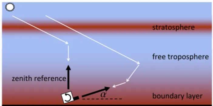
The Multi-Axis Differential Optical Absorption Spec-troscopy (MAX-DOAS) method (e.g. Wagner et al., 2004; H¨onninger et al., 2004; Wittrock et al., 2004; Sinreich et al., 2005; Friess et al., 2006; Leigh et al., 2007; Irie et al., 2008a) offers an alternative in this respect, since it has a much larger spatial representativeness than in situ surface moni-tors. MAX-DOAS instruments observe scattered solar ra-diation from the surface – in the UV and/or Visible – at a spectral resolution of typically 0.5 nm in multiple viewing di-rections (see Fig. 1). Small elevations have a relatively high sensitivity to the lower troposphere, since detected photons at small elevations have longer paths through these layers than photons observed at larger elevations. Radiative trans-fer simulations at 428 nm show that the horizontal represen-tative range is about 5 to 10 km, whereas the vertical range is about 1 to 4 km. Both ranges are wavelength dependent. The horizontal and vertical range also have a strong depen-dence on elevation, see e.g. Wittrock et al. (2004) and Pikel-naya et al. (2007). The increased sensitivity to the lower troposphere also distinguishes the MAX-DOAS technique from other ground-based passive DOAS techniques, such as direct-sun DOAS (total column NO2, see e.g. Herman et al.,

2009), and zenith sky DOAS (stratospheric NO2, see e.g.

Melo et al., 2005).

The various DOAS techniques (see Platt and Stutz, 2008, for an extensive overview) have in common that the analysis of spectral measurements of atmospheric radiation is based on the DOAS equation:

ln

_{I (λ)}

I_ref(λ)

= −

n X

i=1

1σi(λ)1NiS+P (λ). (1)

In this equation n differential cross-section spectra 1σ (λ)i=1,n and a low-order polynomial P (λ) are

fit-ted to the natural logarithm of the ratio of two atmospheric spectraI (λ). A differential cross-section uniquely charac-terizes a trace gas and is obtained by subtracting a low-order polynomial from the cross-section. The two atmospheric spectra in the DOAS equation correspond to two differ-ent viewing directions, or times of observation, or both, depending on the specific DOAS application.

The fitting procedure yields a so-called differential slant column (density) 1NS in [molecules/cm2] for each trace gas. The differential slant column represents the difference in trace gas absorption along the two light paths correspond-ing to the atmospheric spectra. In the case of MAX-DOAS, it is custom to combine a zenith spectrum with a spectrum cor-responding to another, preferably small, elevation α, since

a

stratosphere

free troposphere

boundary layer

Fig. 1. Illustration of DOAS observation. The Mini MAX-DOAS instrument of this study can rotate only in one vertical plane, i.e. it has a fixed azimuth. The viewing direction is referred to as the elevation, which is the angle (α) with the horizontal. For both the DOAS method and relative intensity observations, an observation at elevationαis always combined with a zenith observation (α=90◦). Two examples of photon paths are shown in white. MAX-DOAS observations are relatively insensitive to the trace gases in the strato-sphere, as long as the zenith and non-zenith observations are taken within a time frame where the solar zenith angle changes only little: the sensitivity of the MAX-DOAS observation to NO₂in a particu-lar horizontal layer is proportional to the difference in (detected) photon path length through that layer, between the observations pointed at the zenith and at elevationα.

photons detected at small elevation have the largest path length difference with photons detected in the zenith, and this combination thus gives a high sensitivity to the lower troposphere.

In this study, MAX-DOAS observations are used for the retrieval of tropospheric columns of NO2. To convert a

dif-ferential slant column to a corresponding tropospheric verti-cal columnNTr, a so called differential air mass factor1M is required. This factor is a function of the elevationα– and to a lesser extent of many other parameters – and is defined here as the ratio of the differential slant column density and the tropospheric column density of NO2:

1Mα=

1NS α

NTr . (2)

The simplest calculation of MAX-DOAS differential air mass factors has become known as the geometrical approx-imation (H¨onninger et al., 2004). The geometrical approxi-mation is not based on radiative transfer simulations, but as-sumes that the last scattering altitude of photons detected at the surface is below the stratosphere and above the tropo-spheric layer of a trace gas. This assumption leads to the following relation:

1Mα=

1−sin(α)

Although the geometrical approximation is known to be in-accurate for small elevations (see e.g. Wittrock et al., 2004; Pinardi et al., 2008), this approximation is believed to give an acceptable first estimate of the tropospheric column if ap-plied to a relatively large elevation, such as 30◦. The geo-metrical approximation is used in e.g. Brinksma et al. (2008), Hains et al. (2010) and Wagner et al. (2010).

To exploit the high sensitivity of the MAX-DOAS tech-nique at small elevations, it is desirable to have appropri-ate differential air mass factors for these viewing directions. This requires a more sophisticated description of the radia-tive transfer than the geometrical approximation. Since pho-ton paths through the atmosphere are affected by aerosols, it is essential to take the effect of aerosols on the differential slant columns into account.

Recently developed algorithms to estimate aerosol extinc-tion profiles from MAX-DOAS observaextinc-tions, often depend on MAX-DOAS measurements of O4 absorption (see e.g.

Wagner et al., 2004; Sinreich et al., 2005; Friess et al., 2006; Irie et al., 2008a; Cl´emer et al., 2010). Absorption measure-ments of the collision complex of oxygen molecules, O4, can

be related via inverse modeling to the aerosol extinction pro-file, since O4absorption depends on the photon path length

through the atmosphere on which aerosols have significant impact. The profile shape of O4 is well-known, it has the

shape of the squared pressure profile. 1.3 This paper

In this study, we propose a simple algorithm for a first order aerosol correction on the differential air mass factors as an alternative to the full combined retrieval of NO2and aerosol

extinction profiles based on both O4 and NO2 differential

slant column observations. In our algorithm, aerosol char-acterization, in terms of aerosol optical thickness (AOT), is based on relative intensity measurements. Relative inten-sity observations are defined as the ratio of the sky radi-ance at elevationα and the sky radiance in the zenith, and they have the advantage of a strong dependence on bound-ary layer AOT and almost no dependence on boundbound-ary layer height (Sect. 3.2). This characteristic of relative intensity ob-servations distinguishes it from O4differential slant column

measurements.

The structure of this paper is as follows: first a short de-scription of the instrument is given, together with a character-ization of the field-of-view and slit function (Sect. 2). Also the set-up of the instrument is described, the correction of measured spectra and the settings of the DOAS fit. Radiative transfer modeling of relative intensities and differential air mass factors is described in Sect. 3. A sensitivity study is per-formed, and error sources are discussed. Results of applica-tion of the algorithm to selected days are given in the Sect. 4. Furthermore the applicability of the geometric approxima-tion is discussed, based on both model simulaapproxima-tions and obser-vations. Finally a verification of the aerosol optical thickness

Fig. 2. Measurements with the Mini MAX-DOAS instrument of a Mercury line source at 407.8 [nm], at four different temperatures.

retrieval with AERONET data is shown, and a comparison with tropospheric NO2from the Ozone Monitoring

Instru-ment (OMI).

2 Measurements

2.1 Mini MAX-DOAS instrument

The observations in this study were made with a so-called Mini MAX-DOAS instrument (e.g. H¨onninger et al., 2004; Bobrowski, 2005) produced by Hoffmann GmbH, Germany. This relatively small MAX-DOAS instrument consists essen-tially of a lens, optical fiber and UV/VIS spectrometer, all contained in one metal box that is mounted on a pointing mechanism (stepper motor). The instrument is designed to operate in the open air for long periods in an automated fash-ion. Stabilizing the temperature by cooling is made possible by a Peltier element, which cools up to 25◦C below ambi-ent. Incoming light is focused by a lens (f=40 mm) on the entrance of an optical fiber which is connected to the Ocean Optics “USB2000” crossed Czerny-Turner type spectrome-ter with a Sony “ILX511” CCD detector (2048 pixels). The wavelength range of the instrument is 290 to 433 nm.

Measurements with a monochromatic light source (Mer-cury lamp) were performed (see Fig. 2). These measure-ments indicated that the line shape (slit function) is asym-metric, and has a FWHM of 0.6 nm at around 408 nm. The line shape shows little temperature dependence at this wave-length, which is not far from the spectral fitting window for NO2(Sect. 2.3.2).

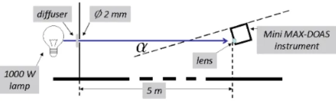
plane of the instrument and the horizontal plane, when the instrument is rotated such that it has maximum signal from a distant light source that is at the same height as the lens of the instrument. The pointing offset was measured each time after the instrument box was opened for maintenance and showed substantial variations (e.g. one occasion with a change from−2.0◦to +0.4◦) due to small displacements of the fiber entrance. The experiment was repeated including a black tube in front of the lens (not drawn), which is used nor-mally to block stray light. Adding the tube did not change the results. The pointing offset was taken into account each time the instrument was started. The pointing of the instrument was checked on a weekly basis.

2.2 Operations

Observations were performed from the roof of the KNMI building in De Bilt, The Netherlands (52.101◦_{N, 5.178}◦_E), from 14 November 2007 until 29 April 2008 and from 11 September 2008 until 21 April 2009 with some days missing due to technical circumstances, resulting in 362 days of ob-servations in total. The azimuth position of the instrument was fixed towards the North-East (at 46◦ _{azimuth relative} to North). This direction was chosen for practical purposes (constraints at small elevations by trees and buildings sur-rounding the measurement site), and to look away from the sun for most of the day throughout the year, which is ad-vantageous with respect to the sensitivity of the retrievals to estimated fixed parameters. Spectra were recorded at 0◦, 2◦, 4◦, 8◦, 16◦, 30◦and 90◦elevation angles. Automated oper-ation of the instrument was done with the DOASIS software developed by IUP Heidelberg in cooperation with Hoffmann GmbH. The integration time for each elevation was set to 30 s divided into multiple shorter scans to prevent the detec-tor from saturation.

2.3 DOAS analysis of spectra

2.3.1 Correction of spectra

Spectra were corrected for a CCD out offset. This read-out offset (or electronic offset, EO) is temperature-dependent and proportional to the number of sub-spectra that are read-out, added and stored as one spectrum. Since the instrument does not have a shutter, it was not possible to do EO and dark current measurements as a part of regular operations.

EO measurements were performed at different tempera-tures by reading out many spectra with minimum integration time under complete dark conditions (e.g. 1000 read-outs at 3 ms, which is the minimal read-out time of the spectrom-eter). These measurements demonstrated that the EO was almost constant over the whole detector range except for the first ten pixels. Since the first hundred pixels of the detec-tor are in the far UV (below 297 nm) they are virtually blind even under atmospheric measuring conditions. A more

de-Fig. 3.Set-up of the field-of-view characterization experiment with a light source in the distance. The angleαdenotes the rotation in the vertical plane relative to a horizontal starting position of 0◦. At this starting position the light source was at the same height above the table as the lens. The experiment was repeated including a black tube in front of the lens (not drawn), which is used normally to block stray light. Adding the tube did not change the results.

tailed analysis showed that pixels 60–80 had an EO level that was within one percent of the offset level in the fitting win-dow used in this study. For this reason the EO correction of each spectrum was based on an average of these pixels. An advantage of this approach is that this EO correction is less sensitive to (unknown) instabilities in the actual temperature of the instrument than if the EO correction would be based on the registered operation temperature, and an EO-temperature calibration done at another time.

It was decided not to apply a dark current (DC) correction. The DC correction depends on temperature, integration time (of each individual sub-scan) and typically shows a strong pixel to pixel variation. It requires a thermally very stable in-strument to be able to correct measured spectra based on lab-oratory measured DC. The instrument was not expected to be thermally stable to such a high degree for the whole period of operation. The effect of applying an inappropriate dark cur-rent correction is comparable to applying no correction. Not applying the dark current correction in the DOAS NO2 fit

will in general lead to somewhat larger fit residuals but not to systematic biases. Tests on temperature-controlled measure-ments, under representative measurement conditions, have shown that differences between including and not including DC-correction was less than 0.1% in the fitted NO2

differen-tial slant column. A possible explanation for this small effect is that the integration time for individual acquisitions was generally small (of the order of 1 s or less), resulting in a low DC, and that the EO correction described here also includes a correction for the average DC. Only the pixel-to-pixel vari-ations on top of this average DC are not accounted for. For other trace gases with smaller tropospheric column amounts the effect of not correcting for DC will be larger.

2.3.2 DOAS fitting

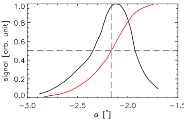
Fig. 4. Field-of-view of the Mini MAX-DOAS instrument, sured with the set-up of Fig. 3. The black curve represents the mea-sured signal at elevationα, and the red curve is the normalized sur-face integral of the black curve. The FWHM is 0.4◦. The center of the field-of-view is defined as the elevation where the red curve equals one half. In this case the pointing offset is−2.16◦.

was selected as a reference, in order to minimize the effect of unknown instrument instabilities on the DOAS fit. Since spectra were measured within 30 s to 2 min from the zenith measurement, the change in stratospheric path length was of relatively little influence, except around sunrise and sunset.

Simulations were performed to study the error introduced by using a semi-simultaneous reference spectrum, as a func-tion of the solar zenith angle. Here equal NO2 column

amounts were assumed for the stratosphere and the tropo-sphere, and no temporal dependence. The error in the NO2

differential slant column is below 1% for solar zenith angles smaller than 74◦_{, and below 5% for solar zenith angles below} 82◦_{. For a representative day in March (around the equinox),} this implies that 8.5 out of 12 h of daylight have an error be-low 1%, and 10.7 h have an error bebe-low 5%.

The cross-sections of NO2(298 K, Vandaele et al., 1997)

O3(243 K, Bogumil et al., 2003) were included in the DOAS

fitting routine as well as the Ring cross-section based on a solar spectrum from Kurucz et al. (1984). Cross-sections were convoluted with the measured instrumental slit function (line shape) of the instrument. The fitting interval was 415 to 431 nm. This interval was chosen because NO2has

rela-tively little interference with other absorbers in this window and because of the relatively pronounced structures in the NO2differential cross-section. It was not possible to exploit

the even more pronounced structures of NO2 between 430

and 450 nm, since those are just outside the detector range of the instrument. Wavelength calibration of the spectra was done in Qdoas by applying a non-linear least squares fit of the spectrum to a high resolution solar spectrum (Kurucz et al., 1984) that was convoluted with the instrumental slit function.

2.4 Relative intensity observations

The observation of relative intensity of skylight is another method to derive information on atmospheric constituents from the MAX-DOAS instrument. Intensity of skylight, I, is measured here as the MAX-DOAS detector signal, cor-rected for electronic-offset (see Sect. 2.3), averaged over a certain spectral interval in one viewing direction. Only rel-ative values of intensity can be compared to their simulated counterparts, since the instrument is not radiometrically cal-ibrated. In this work relative intensity,I_αrel, refers to the ratio of the intensity in directionαto the intensity in the zenith di-rection, where the nearest (in time) zenith spectrum is used: I_αrel= Iα

I₉₀. (4)

The wavelength interval used for I_αrel was 426–429 nm, which is within the NO2DOAS fitting window, and contains

the wavelength chosen for the differential air mass factor cal-culation (Sect. 3.1.3). In the absence of clouds, relative inten-sities in the visible are mainly influenced by Rayleigh scat-tering and aerosol scatscat-tering and absorption. Since Rayleigh scattering is accurately known, relative intensity observa-tions contain information on aerosols, as will be shown in Sect. 3.2.

3 Retrieval algorithm

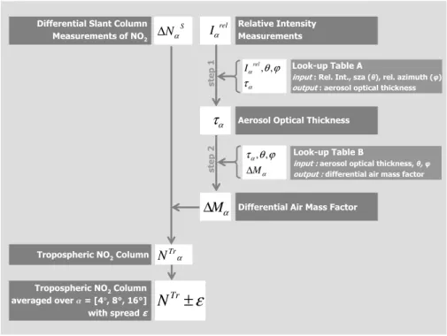
A two step approach is used to derive tropospheric vertical columns of NO2 from MAX-DOAS differential slant

col-umn observations, see Fig. 5. The first step is to estimate aerosol optical thickness from relative intensity observations. This is done by interpolation of the observed relative inten-sity for a particular elevation and solar position (zenith and azimuth) on look-up table values of simulated relative inten-sity as a function of boundary layer AOT. Here it is assumed that both aerosols and tropospheric NO2are homogeneously

distributed in the boundary layer. The second step is to use this estimated AOT in another look-up table containing the NO2differential air mass factors for each elevation and solar

position as a function of AOT.

By this method, the AOT and the tropospheric vertical col-umn of NO2(NαTr) are derived for each elevation independent

of observations in the other elevations. A final NO2

tropo-spheric vertical column (NTr) is found by averaging over the elevations 4◦_{, 8}◦_{and 16}◦_:

NTr=N Tr

4◦+N₈Tr◦+N₁₆Tr◦

3 . (5)

Smaller elevations were not used for several reasons. Firstly, because inhomogeneities in the distribution of aerosols and NO2 in the boundary layer, which are not included in the

S N

α

∆ I rel

α

α α θϕ τ

M ∆

, , α

τ

α Tr

N

α

M

∆

ε

±

N

Differential Slant Column Measurements of NO2

Relative Intensity Measurements

Look-up Table B

input : aerosol optical thickness, θ, φ

output : differential air mass factor Aerosol Optical Thickness

Differential Air Mass Factor

Tropospheric NO2Column

Tropospheric NO2Column

averaged over a_{= [4°, 8°, 16°]}

with spread ε

α α

τ ϕ θ, ,

rel I

ste

p

1

ste

p

2

Look-up Table A

input : Rel. Int., sza (θ), rel. azimuth (φ) output : aerosol optical thickness

Fig. 5.Flow chart of the two-step retrieval algorithm of tropospheric NO₂columns.

will also have the largest effect for the smallest elevations. Thirdly, because the effect of the curvature of the Earth is not captured by the radiative transfer model, which will only have a noticeable effect in the VIS, for small elevations un-der very clear conditions (see also Sect. 3.1.1). Larger ele-vations were not used because the signal-to-noise ratio of the measured differential slant column densities for this eleva-tion was too low, namely often well below 5. This was due to the relative short integration time of 30 s, and the relative low sensitivity of the larger elevations.

As an estimate of the uncertainty on the retrieved average NO2tropospheric column we use the difference between the

maximum and minimum NO2 tropospheric column that is

retrieved for 4◦, 8◦and 16◦elevation (see Sect. 3.3). 3.1 Radiative transfer modeling

A multiple scattering radiative transfer model was used in this study for two purposes. Firstly to derive the look-up ta-bles that relate relative intensity and differential air mass fac-tors to boundary layer AOT. Those look-up tables are used in the retrieval algorithm. Secondly, to study the sensitivity of relative intensities and differential air mass factors to sev-eral parameters that cannot be retrieved and for which fixed (climatological) values are assumed.

The radiative transfer model used in this study is DAK (Doubling-Adding KNMI). The DAK model is based on the doubling-adding algorithm for multiple scattering of sunlight in a vertically inhomogeneous atmosphere with polarization

included (De Haan et al., 1987; Stammes et al., 1989). In the doubling-adding method, one starts with an optically thin layer for which the analytical solution for single and dou-ble scattering suffices to describe the radiation field. Next, subsequent doubling of this optically thin layer to an op-tically thick homogeneous layer, and adding different ho-mogeneous layers together leads to a multi-layered atmo-sphere in which the reflected, transmitted, and internal ra-diation fields are calculated. In each layer, the extinction op-tical thickness, single scattering albedo and phase matrix (or phase function for unpolarized light) have to be prescribed. These atmospheric input parameters are calculated from tem-perature, pressure, trace gas mixing ratio, and aerosol profiles (Stammes, 2001). The inclusion of polarization in comput-ing the radiation fields is especially important in the UV and blue parts of the solar spectrum, where atmospheric Rayleigh scattering is dominating.

3.1.1 Comparison with other radiative transfer models

2007). This deviation at 577 nm was consistent with the other plane parallel models. The same comparison at 360 nm showed no difference between spherical and plane-parallel models.

Based on this comparison it was concluded that the DAK simulations could be applied to the MAX-DOAS observa-tions at around 425 nm for elevaobserva-tions of 4 degrees and above. 3.1.2 Parameter settings

In the algorithm and radiative transfer model, several param-eters were assumed fixed. These are also the standard set-tings in the sensitivity study of Sect. 3.2. These parameters are:

(a) Block functions to describe the aerosol extinction pro-file and NO2 profile in the planetary boundary layer (layer

height: 1.0 km); (b) US-standard mid-latitude summer pro-files for temperature and pressure at all heights and for NO2 above 5 km; (c) NO2 tropospheric vertical column is

2×1016molecules/cm2; (d) Aerosol characterization: sin-gle scattering albedo is 0.92, asymmetry parameter is 0.70, Henyey-Greenstein phase function; (e) Surface albedo is 0.06; (f) Effect of linear polarization is included. The choice for this single scattering albedo and asymmetry parameter was based on AERONET observations from the Cabauw site (22 km from instrument location), for fourteen blue sky days in the years 2007–2009 throughout the various seasons. 3.1.3 Calculation of differential AMF

The differential air mass factor was calculated for one effec-tive wavelength (428.22 nm), and this differential AMF was assumed to be representative for the whole fitting window 415–431 nm. Assumptions with respect to the model atmo-sphere for which differential AMFs and relative intensities were calculated, are described in the previous section.

The differential air mass factor was calculated in a way that is somewhat different from (A) the traditional method (see Platt and Stutz, 2008), and (B) the box-AMF method (see e.g. H¨onninger et al., 2004; Wagner et al., 2007), two methods that can be applied to simulations at a single wave-length. In the case of the traditional method, the AMF is derived from two radiative transfer simulations: one for an atmosphere excluding NO2, and another one for an

atmo-sphere including NO2, assuming a specific vertical

distribu-tion of NO2. Also in the case of the box-AMF method (B),

NO2is added and removed to the simulated atmosphere, but

here only in thin vertical layers, one at a time. For both (A) and (B) the differential AMF (1Mα) for an elevation is found

by subtracting from its AMF (Mα) the zenith-AMF (M90◦). In our study an approach is followed which is numeri-cally equivalent to the traditional method within one per-cent. It was chosen because it closely resembles the MAX-DOAS method, where differential slant columns are de-rived directly from spectra in two viewing directions: one

spectrum measured at elevationαand one zenith reference spectrum. Radiative transfer calculations were performed for just one atmosphere, including an assumed NO2vertical

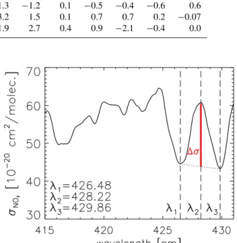
profile. Three wavelengths (426.48, 428.22 and 429.86 nm) were used to be able to subtract a background absorption spectrum, which also includes the low-pass filtered (or broad band) absorption by NO2. In this way, a simulated

tial slant column can be derived from the ratio of the differen-tial absorption slant optical thickness to the differendifferen-tial cross-section of NO2. The three wavelengths were chosen such that

they were close together, at local maximum and minima of the NO2cross-sections, and within the DOAS spectral fitting

window in which the measurements are analyzed (see Fig. 6). The derivation of the differential AMF is as follows. We assume that the light paths in the atmosphere are not changed when adding a relatively weak absorber like NO2. The sky

radiance for elevationαand wavelengthλwith NO2 in the

atmosphere (Iα(λ)) is equal to the sky radiance without NO2

(I_α0(λ)) times an attenuation term depending on the NO2

slant column for this elevation (N_αS), and the NO2

absorp-tion cross-secabsorp-tion (σ (λ)) at this wavelength: Iα(λ)=Iα0(λ)e

−NαSσ (λ)_{, (6)}

also known as the law of Bouguer-Lambert-Beer. Taking the natural logarithm of the ratio of the radiances at elevationα and the zenith (α=90◦_{), and writing:}

R_α(0)(λ)=ln

" Iα(0)(λ)

I₉₀(0)◦(λ)

#

, (7)

and

1N_αS=N_αS−N₉₀S◦, (8)

leads to:

Rα(λ)=Rα0(λ)−1N S

ασ (λ). (9)

This equation may be written for the three wavelengthsλ1=

426.48 nm,λ2=428.22 nm andλ3=429.86 nm.R(α0)andσ

can be interpolated toλ2, using the values atλ1andλ3, which

leads to a second equation defined atλ2. The two equations

atλ2are:

Rα(λ2)=R0α(λ2)−1NαSσ (λ2), (10)

and

R_α∗(λ2)=Rα0∗(λ2)−1NαSσ

∗

(λ2), (11)

where the * refers to the interpolated values atλ₂. Now we assume that in this short interval, R0 can be approximated by a linear function, since it is not affected – in the model atmosphere – by absorbers with a fine-scale structure. Con-sequently:

Table 1. Sensitivity study of eight parameters affecting tropospheric NO₂retrieval: AOT, boundary layer height for NO₂and aerosols (BLH), boundary layer column of NO₂(N), asymmetry parameter of aerosols (ASY), single scattering albedo of aerosols (SSA), surface albedo (ALB), and polarization (POL). Each parameter was changed in the DAK model from case 1 (reference value) to case 2, with all other parameters unchanged. For the elevations 4◦, 8◦and 16◦, the effect of this change is given in percent for the relative intensity (Irel), the differential air mass factor (1M), and for the tropospheric NO₂column retrieved by the two-step algorithm (NTr). The percentage was calculated as follows: [P(case 1)–P(case 2)]/P(case 2)×100%, where, for each line, P(case 2) is the model simulation where only the quantity indicated by the first column of that line was changed to case 2, and where all other parameters were as in case 1. The values in the table therefore represent the error made when the ‘true’ atmosphere would be in a state with one specific parameter as in case 2, whereas this and all other parameters are assumed to be as in case 1 (which corresponds to the settings of the look-up tables described in Sect. 3.1.2). Values were calculated for a solar zenith angle of 60◦and a relative azimuth of 180◦.

α=4◦ α=8◦ α=16◦

change (%) in: change (%) in: change (%) in: param. case 1 case 2 Irel 1M N_αTr Irel 1M N_αTr Irel 1M N_αTr

AOT 0.2 0.4 54 55 0 60 29 0 40 7.4 0

BLH aer.&NO₂[km] 1.0 1.5 −6.5 6.1 −9.7 −3.2 4.2 −4.5 −1.1 1.9 −1.6

BLH NO₂[km] 1.0 1.5 −1.3 23 −19 −0.6 12 −11 −0.1 5.1 −4.5

N[1015molec/cm2] 20 2 −5.7 0.1 −3.8 −4.3 −2.7 1.8 −2.4 −7.7 8.5

ASY 0.70 0.75 −4.8 −3.7 0.15 −5.0 −3.0 1.6 −4.1 −3.1 2.9

SSA 0.92 0.95 −2.1 −0.2 −1.3 −1.2 0.1 −0.5 −0.4 −0.6 0.6

ALB 0.06 0.03 2.7 −0.5 3.2 1.5 0.1 0.7 0.7 0.2 −0.07

POL on off 2.4 0.5 1.9 2.7 0.4 0.9 −2.1 −0.4 0.0

If we define

1Rα(λ2)=Rα(λ2)−Rα∗(λ2), (13)

and

1σ (λ₂)=σ∗(λ2)−σ (λ2), (14)

(see Fig. 6), take the difference of Eqs. (10) and (11), and make use of Eq. (2), we find the following expression for the differential air mass factor (1Mα) at elevationα:

1Mα(λ2)=

1Rα(λ2)

NTr_{1σ (λ} 2)

. (15)

Note from this equation that the differential AMF is calcu-lated only from radiative transfer simulations including NO2,

at three wavelengths, in contrast to the other methods men-tioned at the beginning of this section, where simulations ex-cluding NO2are needed as well, but only at a single

wave-length.

3.2 Sensitivity study

A sensitivity study was performed to quantify the effect of variations in several parameters on the differential air mass factors, relative intensities and the combined steps in the al-gorithm that lead to the retrieved tropospheric NO2column.

These parameters were: boundary layer height, tropospheric NO2 vertical column, aerosol optical thickness, asymmetry

parameter, single scattering albedo, surface albedo and po-larization. In each DAK model run only one parameter was

Fig. 6. Spectrum of the NO₂absorption cross-section convoluted with the instrumental slit function. The three wavelengthsλ₁, λ₂

andλ₃were used in the radiative transfer simulation of the differen-tial AMF and relative intensity. The wavelength range of this figure corresponds to the DOAS spectral fitting window (see Sect. 2.3.2).

changed with respect to the standard settings described in Sect. 3.1.2. The range of the variation of each parameter is given by columns case 1 and case 2 in Table 1.

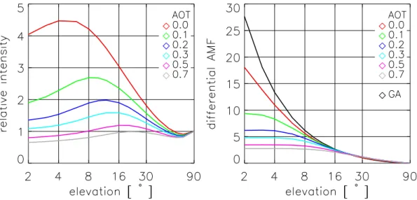
Fig. 7. Radiative transfer simulations with the DAK model of relative intensity (left) and the differential air mass factor of NO₂(right) at 428.22 nm as a function of the elevation, for different values of the AOT. Note the logarithmic scale on the x-axis. The black line in the right plot gives the differential air mass factor for the geometrical approximation (GA). Solar zenith angle = 50◦, relative azimuth angle = 180◦.

of the differential air mass factor. The third column of each elevation shows the sensitivity of the retrieved tropospheric NO2column for that elevation.

Table 1 shows that both the relative intensity and the dif-ferential AMF are most sensitive to the amount of boundary layer aerosols, as seen by the effect of a change in the aerosol optical thickness. The retrieval of tropospheric NO2columns

however, is insensitive to a change in AOT, since the algo-rithm is designed to correct for this change. Figure 7 shows the effect of the AOT on relative intensity and differential AMF in more detail.

The sensitivity to a simultaneous change of both the NO2

and aerosol vertical block profiles is given in the second line of Table 1. This shows that relative intensity observations – and thus the AOT retrieval – are quite insensitive to a change in boundary layer height, when compared with the sensitivity to a change in AOT (first line). However, the combined effect of relative intensity and differential AMF leads to a relatively large change in the tropospheric NO2column, especially for

4◦_{elevation. If only the NO}

2vertical block profile is changed

with respect to the reference situation (third line), then there is a larger change of the differential AMF and the retrieved tropospheric NO2 column. This underlines that knowledge

of the NO2profile shape is crucial to have an accurate

tropo-spheric NO2column retrieval.

Measured differential slant columns are influenced not only by the vertical profile shape of NO2, but also by the

vertical sensitivity to NO2. A useful quantity to describe the

sensitivity to NO2at various altitudes is the height-dependent

air mass factor, a quantity that is also referred to as (differen-tial) box-AMF (see e.g. H¨onninger et al., 2004; Wagner et al., 2007). The height-dependent differential AMF (1mα(z)) at

height z for elevation α, was calculated by perturbing the background NO2profile at heightz:

1mα(z)=

[1Mα]z+−[1Mα]ref

NVz+₋

NVref , (16)

where the superscript “ref” refers to a simulation for a back-ground NO2profile, and the superscriptz+refers to a

sim-ulation where NO2 is added to the background profile at

heightz.

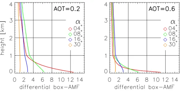
Figure 8 shows the differential box-AMF for different el-evations and for two values of the AOT (see also Wittrock et al., 2004, and Pikelnaya et al., 2007, for similar results obtained with different radiative transfer models). The low elevations have a sensitivity to NO2 that decreases rapidly

with height, whereas the vertical sensitivity of the higher el-evations is more constant. Increasing the amount of aerosols in the boundary layer leads, for the low elevations, to a pro-nounced decrease in sensitivity to NO2with increasing

alti-tude.

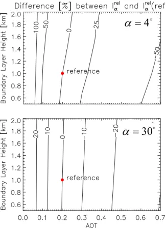
Figure 9 shows the dependence of relative intensity on boundary layer height and aerosol optical thickness, for two elevations (4◦_{and 30}◦_{). The relatively weak sensitivity of} relative intensity to a change in boundary layer height, is the reason that relative intensity observations are more suit-able for boundary layer aerosol optical thickness estimations than measurements of O4, but only in the absence of clouds. A relative intensity observation of only a single elevation is needed to estimate the aerosol optical thickness. O4

Fig. 8. Radiative transfer simulations with the DAK model of height-dependent differential AMF (differential box-AMF) for AOT = 0.2 (left) and AOT = 0.6 (right), at 428.22 nm. Settings in the simulations: boundary layer height for aerosols (block profile): 1.0 km, solar zenith angle = 60◦, relative azimuth angle = 180◦,λ= 428 nm.

From the fourth line in Table 1 it appears that there is an unwanted dependence of the algorithm to the tropospheric NO2 column itself. This can be solved by making the

al-gorithm iterative, with the tropospheric NO2 column as an

additional dimension of the look-up table, but this step was not applied in this study.

Finally, Table 1 shows that the asymmetry parameter, sin-gle scattering albedo, surface albedo and polarization have a relatively small effect on the retrieved tropospheric NO2

column.

Table 1 was calculated for a relative azimuth of 180◦_{and a} solar zenith angle of 60◦_{. Additional studies showed that the} values in the table are representative for other solar positions except when the instrument is viewing in a direction close to the sun (either in viewing directionα, or in the zenith direc-tion) where simulated quantities depend more critically on the aerosol model parameters. Since the Mini MAX-DOAS instrument was pointed towards the North-East, the sun was at relatively large angular distance for most of the time. 3.3 Error sources

There are many possible sources of error in the retrieval of NO2 tropospheric columns from MAX-DOAS

observa-tions. Two types of error may be distinguished: observational errors and modeling errors. The term observational error is used here for all factors leading to an incorrect value for the differential slant column and/or relative intensity.

Systematic error contributions to the observational error are: (1) errors caused by incorrect knowledge of the actual field-of-view, which may be caused by incorrect aiming of the instrument (e.g. when it is unattended after periods of

heavy winds) or by imprecise knowledge of the offset in the field-of-view as described in Sect. 2.1, (2) incorrect elec-tronic offset correction of raw spectra, (3) errors in the differ-ential cross-sections of NO2(e.g. temperature dependency),

(4) errors due to the use of a semi-simultaneous reference spectrum (see Sect. 2.3.2). The DOAS spectral-fitting error represents a mixture of systematic and random errors: incor-rect wavelength calibration of spectra, inaccurate knowledge of instrument slit function, incorrect dark current correction, unknown absorbers, and low signal-to-noise.

The DOAS fitting was performed with a cross section at a fixed temperature (see Sect. 2.3.2). This introduces an error in the differential slant column of NO2 that is proportional

to the temperature difference between the fixed temperature of the cross section used in the fit and the effective tempera-ture of the tropospheric NO2. Although the NO2cross

sec-tion σ_NO2 itself is not strongly temperature dependent, the differential cross section1σ_NO2 shows a much stronger tem-perature dependence: a change in temtem-perature of 20 degrees corresponds to a change inσ_NO2 of 1.6% and to a change in 1σ_NO2 of 7.2%. An estimate of the effective NO2

o

4

=

α

o

30

=

α

Fig. 9.Difference between the modeled relative intensity for a range of AOT and BLH values, and the reference value of relative inten-sity for AOT = 0.2 and a boundary layer height of 1 km (red dot). Two elevations were used in the calculations: 4◦ _{(top) and 30}◦ (bottom). Solar zenith angle = 50◦, relative azimuth angle = 180◦,

λ=428 nm.

The effect of inaccurate estimation of the included model parameters was studied in Sect. 3.2. The algorithm described in this study is most sensitive to the boundary layer height, especially to the vertical profile shape of NO2. This is a

con-sequence of the decrease in sensitivity to NO2with

increas-ing height, especially for low elevations (see e.g. Wittrock et al., 2004, their Fig. 4).

In this study, we estimate the uncertaintyεon the retrieved average NO2tropospheric column (Eq. 5) as the difference

between the maximum and minimum NO2tropospheric

col-umn that is retrieved for 4◦, 8◦and 16◦elevation: ε=maxNTr_[4◦_,8◦_,16◦_]

−minNTr_[4◦_,8◦_,16◦_]

, (17)

where the three tropospheric columns are interpolated to the same point in time. Since the tropospheric columns are de-rived for each elevation independent of the others, this dif-ference, or spread, gives an important indication of the in-ternal consistency of the retrieval. A small spread indicates a consistent retrieval. The spread increases for measurement

conditions that differ from the model atmosphere in the look-up table calculations. For instance, an error in the assumed boundary layer height would lead to different systematic er-rors in the retrieved tropospheric NO2columns for each

el-evation angle (see Table 1). This would result in a system-atic error in the derived average tropospheric NO2 column

and an increase in the spread. The definition of the mea-surement uncertainty includes effects such as: presence of clouds, pointing elevation offsets, horizontal gradients, ver-tical profile shape of aerosols and NO2, and uncertainty due

to a low signal-to-noise.

Since the boundary layer height may well be the parameter with the largest contribution to the uncertaintyεin the tro-pospheric NO2 column retrieval (see Table 1), the two-step

algorithm could be modified by including the boundary layer height as a free parameter, changing it iteratively, by mini-mizingε. However it was decided in this work not to apply this additional step, as the boundary layer height is not the only parameter affectingε, as described above.

Typical values ofεare on average much lower for clear sky than for cloudy conditions (see Sect. 4.1). If data is selected for clear sky conditions, using the criterion that the relative intensity of 4◦, 8◦ and 16◦ is >1, then the median of the measurement uncertainty ε is 2.7×1015molecules/cm2 or 17% relative to a mean tropospheric NO2column of 15.6×

1015molecules/cm2.

4 Results

In this section various results of our new two-step algorithm will be shown. Firstly, several steps in the tropospheric NO2

retrieval algorithm will be illustrated for three selected days, and AOT and tropospheric NO2retrievals will be shown for

four more days. Secondly, the algorithm is compared to the geometrical approximation, which is the default approach to derive tropospheric columns from MAX-DOAS observa-tions. Finally a comparison with AOT from an AERONET instrument and a comparison with OMI tropospheric NO2is

shown.

4.1 AOT and tropospheric NO2for selected days

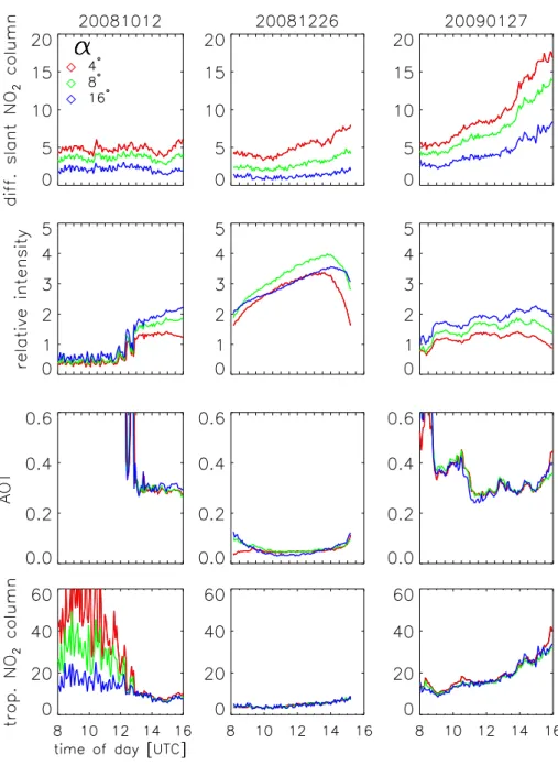
Figure 10 shows the differential slant columns of NO2,

rela-tive intensity, aerosol optical thickness and tropospheric NO2

Fig. 10. Tropospheric NO₂column retrieval for three selected days using the two-step algorithm. All plots have the same time scale on the horizontal axis and in each plot the colors correspond to the elevations indicated by the legend on the upper left. The first row shows the measured NO₂differential slant columns in [1016molecules/cm2]. The second row shows the relative intensities, and the third row the retrieved AOT. The last row shows the retrieved tropospheric column of NO₂in [1015molecules/cm2].

opposite. Under clear sky conditions the intensity of the scat-tered sunlight above the horizon is generally higher than the intensity in the zenith; the maximum intensity occurs usually somewhere betweenα=8◦andα=25◦, depending on e.g. solar position and AOT (see Fig. 7). For this reason relative intensity >1 is a good first indication for clear sky condi-tions, although this is not true in general: for small solar zenith angles the zenith sky may be brighter than the horizon.

Fig. 11.Retrieved aerosol optical thickness (upper row) and tropospheric NO₂column (lower row) for four selected days using the two-step algorithm. The red lines represent the average value of the three elevations: 4◦, 8◦, and 16◦. The spread is indicated by the grey lines.

column retrieval for this day. However, a sudden change be-tween 12:00 and 13:00 UTC cannot be seen in the differential slant columns. This illustrates that differential slant column measurements are mostly sensitive to the lowest kilometers of the atmosphere (whether or not below a cloud). The other two days in Fig. 10 (26 December 2008 and 27 January 2009) are included as an example of both a relatively clean and a relatively polluted day. The clean day, 26 December, was a public holiday with temperatures below 0◦C. It shows stable conditions in both the tropospheric NO2column and AOT.

Four more examples of retrievals for cloud free days are shown in Fig. 11. The spread in the tropospheric columns of NO2 between the three different elevations is relatively

small, about 10%. Possible causes of the spread are dis-cussed in Sect. 3.3.

4.2 Comparison with geometrical air mass factor approximation

The geometrical approximation (GA) of the differential air mass factor for MAX-DOAS observations provides a sim-ple way to determine a first order estimate of the tropo-spheric column of NO2, or other trace gases that are located

primarily in the boundary layer. It is applied to MAX-DOAS observations in e.g. Brinksma et al. (2008) and Hains et al. (2010) in a comparison with other methods to measure tro-pospheric NO2, such as lidar and satellite.

Using the geometric approximation is simple: it does not require an inversion based on radiative transfer modelling. The accuracy of this approximation has been discussed by e.g. H¨onninger et al. (2004), Wittrock et al. (2004), and Pinardi et al. (2008), based on radiative transfer modelling results.

Fig. 12. Difference between the differential air mass factor simu-lated with the DAK radiative transfer model, and the differential air mass factor of the geometrical approximation (GA) for 30◦ eleva-tion, as a function of solar position. AOT = 0.2,λ= 428.22 nm. As an example, the red curve represents the path of the sun trough the sky above De Bilt on 21 March 2009, relative to the viewing az-imuth of the instrument, which was 46◦East from North (sunrise is indicated by “R”, sunset by “S”).

Fig. 13. Retrieved tropospheric NO₂ column in De Bilt for 21 March 2009. The grey band indicates the tropospheric NO₂column retrieval with the two-step algorithm, based on differential slant col-umn measurements atα=4◦, 8◦and 16◦. The red line represents the two step-algorithm applied to 30◦. The blue line is based on the geometrical approximation (GA), also for 30◦elevation. A one-hour running average has been applied to the differential slant col-umn data in order to suppress noise.

GA have almost the same differential air mass factor for 30◦ elevation. However, it can be seen from Fig. 12 that even for this high elevation, the difference between the GA and the model may become as large as 25%, depending on the rel-ative position of the sun, and to a lesser extent on the AOT. At smaller relative azimuths this relative difference is even higher.

The question remains whether the algorithm proposed here, using a combination of lower elevation angles, an aerosol correction and AMFs derived from radiative trans-fer model calculations, gives a more accurate value for the tropospheric NO2column than the GA used on the 30◦

ele-vation measurement.

Figure 13 shows the tropospheric NO2 column derived

from the GA forα=30◦ _{(blue line), and the tropospheric} NO2 column and its estimated uncertainty derived with the

two-step algorithm applied toα=4◦_{, 8}◦_{and 16}◦_{(grey band)} for a clear-sky day. The systematic difference between the two methods for most of this day can be fully explained by the known systematic discrepancies of the GA which does not take multiple scattering, the relative azimuth angle, and the solar zenith angle into account.

This can be seen when looking at the difference between the results of the GA (blue line) and the two-step algorithm applied toα=30◦_{(red line), which directly reflects the} dif-ference in AMFs (see also the red line in Fig. 12). The results of the two-step algorithm atα=30◦ is close to the results for lower elevation angles (grey band), within twice the esti-mated uncertainty. The larger uncertainty between 08:30 and 09:30 a.m. indicates an uncertain retrieval, which is probably caused by a relatively large difference between measurement conditions and one or several parameters that are assumed fixed in the model (e.g. the boundary layer height).

The estimated uncertainty in the tropospheric NO2column

derived with the two-step algorithm is smaller than 15% for most of the day. In Sect. 3.3 it is shown that this uncertainty includes the effect of some major systematic and random er-ror sources, because of the combination of the measurements at three different elevation angles.

It can be concluded that the uncertainty in the results of the two-step algorithm is often smaller than the known sys-tematic discrepancies of the GA. The combination of multi-ple elevations enables an uncertainty estimate, based on the measurement conditions rather than on simulations, which is not possible with the GA: lower elevations than 30◦_cannot be used as they have even larger systematic discrepancies, and higher elevations do not add new information since the vertical sensitivity functions (box-AMF) of those higher el-evations are almost identical to 30◦_{, i.e. they are parallel to} the orange line in Fig. 8.

4.3 Verification of AOT with AERONET data

Fig. 14. Comparison between AOT derived from MAX-DOAS relative intensity observations in De Bilt and AERONET AOT (Cabauw). Both sites were 22 km apart. The selection criteria de-scribed in Sect. 4.3 were applied to all measurements in the obser-vation period (see Sect. 2.2). The red line represents a linear regres-sion, where the squared orthogonal distance of all points to the 1:1 line was minimized.

4.4 Comparison with satellite observations

As a first application of the time series of tropospheric NO2

columns derived from the Mini MAX-DOAS measurements in De Bilt, an inter-comparison was made with tropospheric NO2 data (DOMINO-product, see Boersma et al., 2007)

from the Ozone Monitoring Instrument (OMI, see Levelt et al., 2006). The DOMINO data selection was based on the following criteria: the satellite cloud fraction should be below 0.2 and the NO2 slant column should be

be-low 2×1017molec/cm2. Pixels affected by the OMI row-anomaly were removed. A coincident ground and satellite observation was defined as a measurement where the ground site was within the satellite pixel (which has an approxi-mate rectangular shape, ranging from 13×24 km2_{at nadir}

to 26×135 km2 _{at the edge of the swath, M.R. Dobber et}

al., personal communication, 2009). The ground-based tro-pospheric column was averaged over 15 min around the time of satellite overpass.

A correction was applied to account for the fixed tempera-ture assumed for the NO2cross section (see Sect. 2.3.2). Two

steps were taken to estimate the effective NO2temperature at

the time of observation.

First the difference was determined between the surface temperature and the effective NO2temperatureT_NO2eff :

T_NO2eff =

R

T (z)m(z)n(z)dz R

m(z)n(z)dz , (18)

wherem(z)is the the height-dependent differential air mass factor for an AOT of 0.2 (see Fig. 8),n(z)is a block profile for NO2 from 0–1 km, and T (z)is a standard temperature

profile. A difference of about−2.5◦C was found between the surface temperature and the effective NO2 temperature

for all three elevations 4◦, 8◦and 16◦.

Then surface temperature data were taken from KNMI temperature observations in De Bilt, and from this 2.5◦_{C was} subtracted to determine the effective NO2temperature. The

ratio of1σ (see Fig. 6) at the temperature of the NO2cross

section in the DOAS-fit and1σ at the effective NO2

tem-perature was applied as a temtem-perature correction factor to the MAX-DOAS tropospheric NO2columns.

Figure 15 shows a scatter plot of the comparison. Three different selections of the MAX-DOAS data were made, based on different constraints on the (relative) spread of the ground-based tropospheric column of NO2 (see Table 2).

From 362 days of ground-based observations (see Sect. 2.2) only 123 data points remain after applying the selection cri-teria on the satellite data (including coincidence with the ground-based observation). Only 17 ground-based observa-tions pass the 10% threshold, as described in Table 2.

The table shows that the correlation between the ground-based and satellite data improves with a more strict selection of the ground-based observations. However, when the esti-mated uncertainty (spread) of the ground-based observations is less than 10%, the standard deviation of the differences be-tween the two data sets is about 25% (3.8×1015molec/cm2 for a mean value of about 15×1015molec/cm2).

To test if the spread between the OMI and the MAX-DOAS tropospheric NO2 columns is dominated by the

es-timated retrieval errors from both data sets, a χ2 test was applied:

χ_ν2= 1

N N X

i=1

(xi−yi)2 ε2

xi+ε

2 yi

, (19)

whereN is the number of data points (xi,yi),xi is an OMI

tropospheric NO2column measurement, with retrieval error

εxi, andyi is a MAX-DOAS tropospheric NO2column mea-surement with retrieval errorεyiestimated from the spread as described in Eq. (17). For the three selections of the data, as described in Table 2,χ_ν2is between 2.5 and 3. Assuming an average difference of zero between the data sets and normal error distributions, the probability of exceeding these values forχ_ν2is less than 0.1%. Hence, the spread is larger than can be expected from the estimated retrieval errors alone.

A possible explanation for the part of the spread that is not explained by the retrieval errors, is the difference in ob-servation techniques. First, the spatial representativity of the two types of observation is quite different. The hori-zontal footprint of an OMI pixel is different from the hor-izontal domain of the MAX-DOAS observation. Whereas OMI samples a domain of>300 km2_{, the MAX-DOAS has}

Table 2.Comparison between OMI and MAX-DOAS tropospheric NO₂. The three rows represent three different sets of selection criteria that are applied to the ground-based retrieved tropospheric NO₂columns. Each set consists of an upper limit of the relative measurement uncertainty (εrel_MDin percent) and an upper limit of the absolute measurement uncertainty (εabs_MDin 1015molec/cm2). A point is selected if it satisfies one or both of the limits. The other columns are: number of collocations that satisfies these criteria (n), correlation (R), mean difference (< d >in 1015molec/cm2), standard deviation of differences (σ<d>) in 1015molec/cm2, slope (sfit) of linear fit that minimizes

the sum of the squared orthogonal distances,y-axis offset of this linear fit (o_fitin 1015molec/cm2), mean relative and absolute measurement uncertainty of the ground based observations (< εrel_MD>in percent and< εabs_MD>in 1015molec/cm2), and the same quantities for the satellite observation: (< ε_OMIrel >and< εabs_OMI>).

Selection criteria Comparison OMI – MAX-DOAS

set εrel_MD εabs_MD n R < d > σ<d> sfit ofit < εMDrel > < εabsMD> < εOMIrel > < εOMIabs >

1 ≤30% ≤3 76 0.64 −2.1 7.6 1.21 −0.5 23% 2.8 59% 6.3

2 ≤20% ≤2 48 0.73 −1.0 6.2 1.0 1.2 20% 2.0 60% 6.8

3 ≤10% ≤1 17 0.88 0.6 3.9 0.8 1.2 22% 0.9 57% 6.4

the lowest elevation of 4◦_{. Also the vertical range that} con-tributes to the tropospheric NO2 signal is different for the

satellite and the MAX-DOAS observations. The sensitivity of MAX-DOAS to NO2 decreases quickly with increasing

height of NO2, especially for high aerosol loads (see Fig. 8),

whereas the satellite has increasing sensitivity with increas-ing NO2height (Eskes and Boersma, 2003). Consequently,

the relative contribution of the free-tropospheric NO2to the

total tropospheric NO2 differs between the satellite and the

MAX-DOAS.

Separation of the free tropospheric and boundary layer contribution to the tropospheric NO2column requires

accu-rate knowledge of the NO2profile shape, both for the

satel-lite and the MAX-DOAS retrieval. Lack of knowledge of the vertical distribution of NO2 thus complicates the

com-parison of satellite and MAX-DOAS NO2-data as well as the

interpretation of satellite retrievals in terms of surface con-centrations.

More observations and understanding of vertical profiles of NO2are needed to study the variety of circumstances

un-der which differences between satellite and ground-based ob-servations occur.

5 Conclusions

We described a new two-step algorithm to retrieve aerosol corrected tropospheric NO2columns from MAX-DOAS

ob-servations.

We used relative intensity observations performed with a mini MAX-DOAS instrument to estimate the aerosol opti-cal thickness of the boundary layer. Based on this AOT-estimation, aerosol corrected differential air mass factors for NO2 were determined to convert differential slant columns

of NO2to tropospheric columns.

Fig. 15. Comparison between tropospheric NO₂ columns from MAX-DOAS observations in De Bilt and OMI (DOMINO product). The selection of data-points is described in Table 2 (MAX-DOAS), and Sect. 4.4 (OMI), and was applied to all measurements in the observation period (see Sect. 2.2). The selection described in the first row of Table 2 includes all points in the plot, the selection de-scribed in the second row includes all black and red points, and the selection of the last row includes only the red points.

Relative intensity measurements have a strong dependence on boundary layer AOT and almost no dependence on bound-ary layer height although this dependence increases slightly with decreasing elevation.

NO2in the algorithm. An uncertainty estimate in the results

is derived from the spread in the tropospheric NO2columns

that are derived independently for each elevation (4◦_{, 8}◦_and 16◦). A low spread indicates a consistent retrieval of the tro-pospheric NO2column for the three elevations.

The use of the relatively low elevations makes the retrieval method more sensitive to trace gases in the boundary layer than the often used geometrical approximation that can only be applied at higher elevations (30◦_{). The geometrical air} mass factor approximation for 30◦_{elevation gives a good first} estimate of the tropospheric column. However, even for this high elevation, the differential air mass factor of the geomet-rical approach may differ up to 25% from the differential air mass factors using radiative transfer modeling. For relative azimuths smaller than 40◦_{, this difference may even be larger.} The relatively low-cost (Mini) MAX-DOAS instruments are capable of generating long time-series of tropospheric composition data in an automated fashion. MAX-DOAS ob-servations are particularly valuable for the purpose of satel-lite validation of tropospheric trace gases due to the hori-zontal and vertical range where trace gases can be detected, which is on the order of 1 to 4 km in the vertical and 5 to 10 km in the horizontal, depending on the AOT. Accurate comparison of satellite and ground-based observations re-quires knowledge of the NO2 profile shape, in order to

ac-count for differences in the sensitivity to NO2 at different

heights.

The two-step retrieval scheme presented here was applied to cloud-free periods in a twelve month data set of MAX-DOAS observations in De Bilt, The Netherlands, between Autumn 2007 and Spring 2009 (summer of 2008 not in-cluded). For cloud free periods, the average tropospheric NO2 column was 15.6×1015molecules/cm2. The median

of the estimated relative uncertainty was 17%.

In a comparison with AERONET (Cabauw site, 22 km from De Bilt) a mean difference in AOT (AERONET minus MAX-DOAS) of−0.01±0.08 was found, and a correlation of 0.85.

Tropospheric NO2 columns were compared with OMI

satellite tropospheric NO2. Only satellite pixels over De

Bilt were selected. The spread in the tropospheric NO2

columns retrieved (semi)-simultaneously from the different MAX-DOAS elevations was used as a selection criterion. For ground-based observations restricted to a spread below 10%, a correlation of 0.88 was found, and no significant dif-ference. The spread between OMI and MAX-DOAS tropo-spheric NO2column measurements is larger than can be

ex-pected from the estimated retrieval errors alone. This may be due to differences in the spatial representativity of the two observation techniques.

Acknowledgements. The authors greatly acknowledge the anony-mous reviewers for carefully reading the manuscript and for giving constructive comments and suggestions.

The authors would like to thank M. Van Roozendael, C. Fayt and G. Pinardi from the Belgian Institute for Space and Aeronomy (IASB/BIRA) for providing the Qdoas software that was used for the DOAS analysis, and for giving valuable support and advice.

Furthermore we would like to thank S. Kraus and T. Lehmann of the Institute for Environmental Physics at the University of Heidelberg for providing the DOASIS software package.

We would like to thank K. F. Boersma, J. de Haan, M. Allaart and M. Dobber for useful discussions on this study.

We acknowledge the free use of tropospheric NO₂ column data from the OMI sensor from www.temis.nl.

We acknowledge the efforts of the AERONET team, and in partic-ular the TNO team lead by G. de Leeuw for the measurement and provision of AOT data.

Finally, we acknowledge the support of the European Commission through the GEOmon (Global Earth Observation and Monitoring) Integrated Project under the 6th Framework Program (contract num-ber FP6-2005-Global-4-036677).

This work has been financed by User Support Program Space Research via the project “Atmospheric chemistry instrumentation to strengthen satellite validation of CESAR” (EO-091).

Edited by: C. Senff

References

Blond, N., Boersma, K. F., Eskes, van der A, R. J., Van Roozendael, M., De Smedt, I., Bergametti, G., and Vautard, R.: Intercompari-son of SCIAMACHY nitrogen dioxide observations, in situ mea-surements and air quality modeling results over Western Europe, J. Geophys. Res., 112, D10311, doi:10.1029/2006JD007277, 2007.

Bobrowski, N.: Volcanic Gas Studies by Multi Axis Differential Optical Absorption Spectroscopy, Ph.D. thesis, University of Heidelberg, Germany, 2005.

Boersma, K. F., Eskes, H. J., and Brinksma, E. J.: Error analysis for tropospheric NO₂ retrieval from space, J. Geophys. Res., 109, D04311, doi:10.1029/2003JD003962, 2004.

Boersma, K. F., Eskes, H. J., Veefkind, J. P., Brinksma, E. J., van der A, R. J., Sneep, M., van den Oord, G. H. J., Levelt, P. F., Stammes, P., Gleason, J. F., and Bucsela, E. J.: Near-real time retrieval of tropospheric NO₂from OMI, Atmos. Chem. Phys., 7, 2103–2118, doi:10.5194/acp-7-2103-2007, 2007.

Boersma, K. F., Jacob, D. J., Eskes, H. J., Pinder, R. W., Wang, J., and van der A, R. J.: Intercomparison of SCIAMACHY and OMI tropospheric NO₂columns: Observing the diurnal evolu-tion of chemistry and emissions from space, J. Geophys. Res., 113, D16S26, doi:10.1029/2007JD008816, 2008.