TCD
9, 6581–6626, 2015Glaciological and geodetic mass
balance of ten long-term glaciers in
Norway
L. M. Andreassen et al.
Title Page
Abstract Introduction
Conclusions References
Tables Figures
◭ ◮
◭ ◮
Back Close
Full Screen / Esc
Printer-friendly Version
Interactive Discussion
Discussion
P
a
per
|
Discussion
P
a
per
|
Discussion
P
a
per
|
Discussion
P
a
per
|
The Cryosphere Discuss., 9, 6581–6626, 2015 www.the-cryosphere-discuss.net/9/6581/2015/ doi:10.5194/tcd-9-6581-2015
© Author(s) 2015. CC Attribution 3.0 License.
This discussion paper is/has been under review for the journal The Cryosphere (TC). Please refer to the corresponding final paper in TC if available.
Glaciological and geodetic mass balance
of ten long-term glaciers in Norway
L. M. Andreassen, H. Elvehøy, B. Kjøllmoen, and R. V. Engeset
Section for Glaciers, Ice and Snow, the Norwegian Water Resources and Energy Directorate (NVE), Oslo, Norway
Received: 3 November 2015 – Accepted: 5 November 2015 – Published: 26 November 2015
Correspondence to: L. M. Andreassen (lma@nve.no)
TCD
9, 6581–6626, 2015Glaciological and geodetic mass
balance of ten long-term glaciers in
Norway
L. M. Andreassen et al.
Title Page
Abstract Introduction
Conclusions References
Tables Figures
◭ ◮
◭ ◮
Back Close
Full Screen / Esc
Printer-friendly Version
Interactive Discussion
Discussion
P
a
per
|
Discussion
P
a
per
|
Discussion
P
a
per
|
Discussion
P
a
per
|
Abstract
The glaciological and geodetic methods provide independent observations of glacier mass balance. The glaciological method measures the surface mass balance, on a seasonal or annual basis, whereas the geodetic method measures surface, internal and basal mass balances, over a period of years or decades. In this paper, we
re-5
analyse the 10 glaciers with long-term mass balance series in Norway. The reanalysis includes (i) homogenisation of both glaciological and geodetic observation series, (ii) uncertainty assessment, (iii) estimates of generic differences including estimates of in-ternal and basal melt, (iv) validation, and (v) partly calibration of mass balance series. This study comprises an extensive set of data (454 mass balance years, 34 geodetic
10
surveys and large volumes of supporting data, such as metadata and field notes). In total, 21 periods of data were compared and the results show discrepancies be-tween the glaciological and geodetic methods for some glaciers, which in part are attributed to internal and basal ablation and in part to inhomogeneity in the data pro-cessing. Deviations were smaller than 0.2 m w.e. a−1 for 12 out of 21 periods.
Calibra-15
tion was applied to seven out of 21 periods, as the deviations were larger than the uncertainty.
The reanalysed glaciological series shows a more consistent signal of glacier change over the period of observations than previously reported: six glaciers had a significant mass loss (14–22 m w.e.) and four glaciers were nearly in balance. All glaciers have
20
lost mass after year 2000.
More research is needed on the sources of uncertainty, to reduce uncertainties and adjust the observation programmes accordingly. The study confirms the value of carry-ing out independent high-quality geodetic surveys to check and correct field observa-tions.
TCD
9, 6581–6626, 2015Glaciological and geodetic mass
balance of ten long-term glaciers in
Norway
L. M. Andreassen et al.
Title Page
Abstract Introduction
Conclusions References
Tables Figures
◭ ◮
◭ ◮
Back Close
Full Screen / Esc
Printer-friendly Version
Interactive Discussion
Discussion
P
a
per
|
Discussion
P
a
per
|
Discussion
P
a
per
|
Discussion
P
a
per
|
1 Introduction
Glacier mass balance observations are important for studies of climate change, water resources and sea level rise (e.g. IPCC, 2013). Mass balance is the change in mass of a glacier over a stated span of time (Cogley et al., 2011). The mass balance is the sum of surface, internal and basal mass balance components. In situ observations of
5
glacier surface mass balance is called theglaciological method(the terms direct, tra-ditional or conventional method are also used in the literature) where mass balance is measured at point locations, and data are interpolated over the entire glacier surface to obtain glacier-wide averages. Surface mass balance is the sum of surface accumu-lation and surface abaccumu-lation and includes loss due to calving. Mass balance can also
10
be assessed indirectly by the geodetic method (also called cartographic) where the cumulative mass balance for a period is calculated by differencing digital terrain mod-els (DTMs) and converting the volume change to mass using a density conversion. Whereas the glaciological method measures the surface mass balance, the geodetic method measures the sum of surface, internal and basal mass balances. For a direct
15
comparison of glaciological and geodetic balances methodological differences must be considered, such as differences in survey dates (account for ablation or accumulation between the survey dates) and surveyed areas (using the same area and ice divides in both methods). In addition, effects of changes in density profiles between the geodetic surveys must be accounted for. Moreover, recent studies have shown that internal and
20
basal melt may be substantial for temperate glaciers, in particular for maritime high-precipitation glaciers that span large elevation ranges (Alexander et al., 2011, 2013; Oerlemans, 2013).
Comparison of glaciological and geodetic results have revealed both discrepancies and agreements (Cogley, 2009). Several studies on homogenization of mass balance
25
TCD
9, 6581–6626, 2015Glaciological and geodetic mass
balance of ten long-term glaciers in
Norway
L. M. Andreassen et al.
Title Page
Abstract Introduction
Conclusions References
Tables Figures
◭ ◮
◭ ◮
Back Close
Full Screen / Esc
Printer-friendly Version
Interactive Discussion
Discussion
P
a
per
|
Discussion
P
a
per
|
Discussion
P
a
per
|
Discussion
P
a
per
|
Balance” at the Tarfala Research Station in northern Sweden in 2012 describes a stan-dard procedure for reanalysing mass balance series (Zemp et al., 2013), based on best practices. The reanalysis procedures includes homogenization of glaciological and geodetic balances, assessment of uncertainty, validation, and calibration, if nec-essary. It also recommended that mass balance series longer than 20 years should be
5
reanalysed in any case.
Homogenization of mass balance series can be defined as the procedure to correct artefacts and biases that are not natural variations of the signal itself but originate from changes in instrumentation or changes in observational or analytical practice (Cog-ley et al., 2011). In the glaciological method, common inhomogeneities are change in
10
method (e.g. from contour line to altitude-profile method), change in observational net-work, use of different glacier basins and changes in area and elevation over time. In the geodetic method, inhomogeneity may stem from surveys using different sources and methods (e.g. from analogue contour lines to digital point clouds), orientation of the data set, and software. When calculating the geodetic balance it is important that
15
independent data or stable terrain outside the glaciers are used to check the individual DTMs. DTMs should be co-registered (Kääb, 2005) or even reprocessed from original survey data if needed (Koblet et al., 2010). Uncertainty is not only dependent on the standard error of the individual elevation differences, but is also dependent on the size of the averaging area and the scale of the spatial correlation (Rolstad et al., 2009).
20
In Norway, the contribution of glacier melting to runoff instigated systematic mass balance studies on several glaciers from the 1960s. Mass balance programmes have been conducted on more than 40 glaciers for shorter or longer periods (Andreassen et al., 2005; Kjøllmoen et al., 2011).
In this paper, we compare homogenised glaciological and geodetic mass balance for
25
TCD
9, 6581–6626, 2015Glaciological and geodetic mass
balance of ten long-term glaciers in
Norway
L. M. Andreassen et al.
Title Page
Abstract Introduction
Conclusions References
Tables Figures
◭ ◮
◭ ◮
Back Close
Full Screen / Esc
Printer-friendly Version
Interactive Discussion
Discussion
P
a
per
|
Discussion
P
a
per
|
Discussion
P
a
per
|
Discussion
P
a
per
|
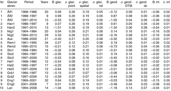
of both glaciological and geodetic observation series, (ii) uncertainty assessment, (iii) estimates of generic differences including estimates of internal and basal melt, (iv) validation, and (v) partly calibration of mass balance series.
A large set of metadata, observations, calculations and procedures were analysed: 454 years of glaciological mass balance data, 34 geodetic surveys/maps and 21
pe-5
riods of concurrent data. The analysed glaciers covered an area of 134 km2 ranging from 60.5 to 70.1◦N.
2 Study glaciers
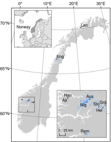
The ten glaciers selected for this study all have long-term mass-balance programmes and geodetic surveys that cover (the larger part of) the period with annual
measure-10
ments (Table 1, Fig. 1). Glaciers with short-term series without concurrent geode-tic surveys are not considered here. The glaciological series are continuous, except Langfjordjøkelen where glaciological measurements are lacking for two years (1994, 1995). The longest series is Storbreen where measurements began already in 1949, the shortest series are for Hansebreen, Austdalsbreen and Langfjordjøkelen where
15
measurements began late in the 1980s (Table 1). All glaciers are part of a glacier com-plex (thus, sharing border with at least one other glacier flow unit), except for Storbreen (Andreassen et al., 2012b). The glaciers in southern Norway are located along a west– east transect, extending from a wet maritime climate where Ålfotbreen and Hansebreen are located to drier conditions in the interior where Gråsubreen is located (Fig. 1).
20
Engabreen and Langfjordjøkelen are located near the coast in the central and northern parts of Norway, and represents the glaciers with the lowest minimum and maximum elevation respectively. The glaciers range greatly in size from 2.2 km2(Gråsubreen) to 46.6 km2(Nigardsbreen). One glacier, Austdalsbreen, is calving into a regulated lake.
The study glaciers have all reduced in volume and area during the past century. The
25
TCD
9, 6581–6626, 2015Glaciological and geodetic mass
balance of ten long-term glaciers in
Norway
L. M. Andreassen et al.
Title Page
Abstract Introduction
Conclusions References
Tables Figures
◭ ◮
◭ ◮
Back Close
Full Screen / Esc
Printer-friendly Version
Interactive Discussion
Discussion
P
a
per
|
Discussion
P
a
per
|
Discussion
P
a
per
|
Discussion
P
a
per
|
during the past 50 years, most so for Langfjordjøkelen (Andreassen et al., 2012a). The other six glaciers are maritime ice cap outlets, that had a mass surplus mainly due to higher snow accumulation in the 1990s, but all have lost mass since 2000 (Andreassen et al., 2005, 2012b; Kjøllmoen et al., 2011). There is significant variability in the mass turnover between the study glaciers, from annual accumulation/ablation of about 1–
5
2 m w.e. for the interior glaciers to 3–6 m w.e. for the maritime glaciers on the West coast (Andreassen et al., 2005).
3 Data and methods
In this chapter we describe the data and methods used for calculating glaciological and geodetic mass balance and for the reanalysis undertaken. We describe the original
10
data sets, the homogenization of these and give uncertainty assessments of systematic and random errors.
3.1 Glaciological mass balance
3.1.1 Surface mass balance observations
NVE’s surface mass-balance series contain annual (net), winter and summer balances.
15
Details on observation programme including maps of the annual monitoring network are found in NVE’s report series Glaciological investigations in Norway (e.g., Kjøllmoen and others, 2011, all reports are available at http://www.nve.no/glacier). Methods used to measure mass balance in field have in principle remained unchanged over the years, although the amount of measurements has varied (Andreassen et al., 2005). The
win-20
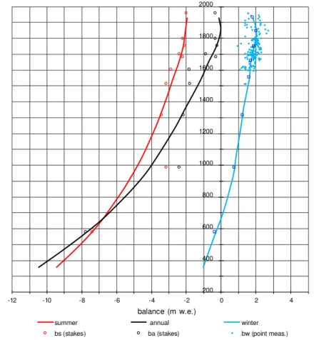
ter balance is measured in spring by probing to the previous year’s summer surface along regular profiles or grids, typical values being 50–150 probings on each glacier every year (Fig. 2). Snow density is measured in pits and with coring at one or two locations at different elevations on each glacier. Stake readings and snowdepth cor-ings are used to verify the probcor-ings. Summer and annual balances are obtained from
TCD
9, 6581–6626, 2015Glaciological and geodetic mass
balance of ten long-term glaciers in
Norway
L. M. Andreassen et al.
Title Page
Abstract Introduction
Conclusions References
Tables Figures
◭ ◮
◭ ◮
Back Close
Full Screen / Esc
Printer-friendly Version
Interactive Discussion
Discussion
P
a
per
|
Discussion
P
a
per
|
Discussion
P
a
per
|
Discussion
P
a
per
|
stake measurements. The number of stake positions varies from glacier to glacier and through time, typical values being 5–15. At Austdalsbreen the annual calving from the glacier is calculated from measured ice velocity near the terminus, surveyed autumn terminus positions and estimated mean ice thickness (Elvehøy, 2011) following Funk and Rötlisberger (1989).
5
To calculate winter (Bw), summer (Bs) and annual (Ba) balances, the point measure-ments are interpolated to area-averaged values. In the first years this was done by the contour line method, since the mid/end of the 1980s this has been done using the profile method. The shift in method was mainly a consequence of a reduction of the observing network on many of the maritime glaciers. In the contour line method
10
the point measurements were plotted on a map and isolines of mass balance were drawn for both winter and summer balances (Fig. S1 in the Supplement). The areas between adjacent isolines within each altitude interval (50 or 100 m) were integrated using a planimeter, and the total amount of accumulation and ablation was calculated for each altitude interval. In the profile method the point measurements vs. altitude are
15
plotted and interpolated balance profiles are drawn to obtain mass balance values for each altitudinal interval (Fig. 3). The elevation of point measurements and area distri-bution are taken from the most recent map/digital terrain model of the glacier. When a new map has been constructed, it was used for the calculations from then and on-wards. However, it may be considerable time lags (up to 30 years) between the mass
20
balance year and the reference area used for calculating mass balances.
Glaciological balances are reported as conventional surface balances, i.e. internal and basal balances have not been part of the observational programme and are not accounted for in the published mass balance records.
3.1.2 Homogenization of surface mass balance
25
TCD
9, 6581–6626, 2015Glaciological and geodetic mass
balance of ten long-term glaciers in
Norway
L. M. Andreassen et al.
Title Page
Abstract Introduction
Conclusions References
Tables Figures
◭ ◮
◭ ◮
Back Close
Full Screen / Esc
Printer-friendly Version
Interactive Discussion
Discussion
P
a
per
|
Discussion
P
a
per
|
Discussion
P
a
per
|
Discussion
P
a
per
|
four of the glaciers (Nigardsbreen, Engabreen, Ålfotbreen and Hansebreen), as the first comparison of geodetic and glaciological balances indicated rather large discrepancies between the methods. This detailed homogenisation process included going through the data material for each year to search for inhomogeneities and possible biases in the data calculations. The process included digitisation of point measurements,
recal-5
culating the mass balance using homogenized drainage divides, density conversion, and recalculating from contour to profile method for the earlier years. For the other six glaciers, a less detailed procedure was followed, typically including homogenization of the drainage divide and area–altitude distributions. For Austdalsbreen the calculation procedure of losses due to calving was also homogenized.
10
In the following, we describe in more details the homogenization of the area–altitude distribution, the change from the contour map method to the profile method, and the calving of Austdalsbreen.
Area-altitude distribution
The annual mass-balance calculations were based on a series of maps for each glacier.
15
When a new map or DTM became available some time after the survey the mass-balance was calculated from then on using the new map for the stake and sounding elevations and the area–altitude distribution. The changing glacier area and elevation over time is an inhomogeneity common to all mass balance glaciers (Holmlund et al., 2005; Zemp et al., 2013). To minimize the effects of the changing elevation distribution
20
on the results we obtained glacier wide balance values by recalculating the mass bal-ance for the period of record using both area–altitude distributions. Two approaches were tested, (1) shift: simply using the older map for first half of the period and then using the newer map for the second half, or (2) linear weighting: calculatingBa for all years in the period using both area–altitude distributions and linearly time-averaging
25
between them.
TCD
9, 6581–6626, 2015Glaciological and geodetic mass
balance of ten long-term glaciers in
Norway
L. M. Andreassen et al.
Title Page
Abstract Introduction
Conclusions References
Tables Figures
◭ ◮
◭ ◮
Back Close
Full Screen / Esc
Printer-friendly Version
Interactive Discussion
Discussion
P
a
per
|
Discussion
P
a
per
|
Discussion
P
a
per
|
Discussion
P
a
per
|
trend in glacier change. Langfjordjøkelen is the glacier with the strongest thinning and retreat of the 10 study glaciers (Andreassen et al., 2012a), and is expected to have the largest sensitivity to the DTM used on the mass balance results. A comparison between the two methods for Langfjordjøkelen and Storbreen shows that the difference between method 1 and 2 is small for the cumulativeBa for both glaciers,−0.18 m w.e.
5
for Langfjordjøkelen for the period 1995–2008 and 0.01 m w.e. for Storbreen for the period 1998–2009 (Table 3). Results further reveal that the difference in Ba values for individual years varied between 0.09 and −0.06 m w.e. for Langfjordjøkelen and between 0.01 and−0.02 m w.e. for Storbreen. For simplicity, approach (1) was used for most glaciers. For glaciers with strongly non-linear changes, normalized front variation
10
series might be used to weight the inter-annual area changes (Zemp et al., 2013), but this was not used in this study.
Contour map to profile method
In the 1980s a simplification of the observation programme was carried out after sta-tistical analysis of the previous years’ accumulation and ablation patterns, especially
15
at large outlet glaciers like Nigardsbreen and Engabreen (Andreassen et al., 2005). The interpolation method was also shifted from contour to profile method at the end of the 1980s. However, the profile method can be sensitive to the altitudinal cover-age and the spatial pattern of observations (Escher-Vetter, 2009). Usually the profile method have been used by drawing the area–altitude mass balance curves manually
20
for our mass balance data. To test the sensitivity of the manual drawing on the mass balance results, two of the authors used the point data for Engabreen to draw curves for seven years, 2002–2008. In this period, the glacier had only one stake at the tongue at∼300 m a.s.l. and then about 6 stakes on the ice plateau from∼950 to 1350 m a.s.l. The profile curves were then compared with the curves drawn manually by the
princi-25
TCD
9, 6581–6626, 2015Glaciological and geodetic mass
balance of ten long-term glaciers in
Norway
L. M. Andreassen et al.
Title Page
Abstract Introduction
Conclusions References
Tables Figures
◭ ◮
◭ ◮
Back Close
Full Screen / Esc
Printer-friendly Version
Interactive Discussion
Discussion
P
a
per
|
Discussion
P
a
per
|
Discussion
P
a
per
|
Discussion
P
a
per
|
little sensitivity to the subjective judgement in the manual drawing of the annual curves in the profile method.
Calving
At Austdalsbreen, a map from 1966 was originally used for 1988–2008 and the map from 2009 since 2009. In the homogenization, mass balance was recalculated using
5
the 2009 ice divide for all years, the 1988 glacier outline and area–altitude distribution for 1988–1998, and the 2009 outline and area–altitude distribution from 1999. Due to construction of a hydropower reservoir in front of Austdalsbreen in 1988–1989, the lake level was changed from a fixed level around 1156 m a.s.l. to a lake level varying between 1150 and 1200 m a.s.l. The lowest part of the glacier calved offduring the first
10
two years. Thus, in the homogenization this was accounted for by removing the calved offpart below 1200 m a.s.l. (0.093 km2) from the area–altitude distribution from 1990. As part of the homogenization, the annual calving volumes were also recalculated.
3.1.3 Example: homogenization of the Nigardsbreen surface mass balance
record
15
Nigardsbreen has been subject for annual glaciological mass balance measurements since 1962 (Østrem and Karlén, 1962). NVE has carried out the measurements in all years, but many people have been involved in the field work during this period, also the principal investigator responsible for the calculations have changed several times in this period. The original published results show positive mass balance from 1962 to 1988,
20
a large surplus from 1988 to 2000 and near balance (a small deficit) from 2001 to 2013. Detailed glacier maps have been constructed from aerial photographs taken in 1964, 1966/74 (combined) and 1984, and by laser scanning in 2009 and 2013. The original glaciological mass balance series were compared with geodetic mass balance for the periods 1964–1984, 1984–2013 and 2009–2013, and revealed larger discrepancies.
25
TCD
9, 6581–6626, 2015Glaciological and geodetic mass
balance of ten long-term glaciers in
Norway
L. M. Andreassen et al.
Title Page
Abstract Introduction
Conclusions References
Tables Figures
◭ ◮
◭ ◮
Back Close
Full Screen / Esc
Printer-friendly Version
Interactive Discussion
Discussion
P
a
per
|
Discussion
P
a
per
|
Discussion
P
a
per
|
Discussion
P
a
per
|
a new digital point cloud was constructed from the 1964 photos in 2014. The combined 1966/74 map was made using photos from the two years, and due to the large time gap between the photos and uncertainties in which parts mapped by which photos, the map was not used for the geodetic calculations.
All point measurements of snow depths and stakes were identified in data reports
5
and maps, and given positions and altitudes from the relevant DTM. The re-calculation was based on the profile method within the hydrological basin and with the current DTM and ice divide from 2009/13. The review of the historic data sets and the re-calculation process also revealed some errors in the original mass balance calculations in some years, e.g. the handling of summer snow fall and density conversions. These errors
10
were corrected in the re-calculations.
The glaciological mass balance methodology has changed through the period of measurements. Five types of inhomogeneities were identified and accounted for in the homogenisation (Table S1 in the Supplement).
Contour line method
15
From 1962 to 1988, both winter and summer balances were calculated using the con-tour line method. From 1989, the altitudinal mass balance curves were constructed by plotting point measurements vs. altitude. Accordingly, the homogenization involved re-calculation of the period 1962–1988 using the profile method. The curves were man-ually drawn between the point measurements.
20
Area-altitude distribution
The original mass balance calculations were based on area–altitude distribution from five maps (1964, 1974, 1984, 2009 and 2013). There were considerable time lags be-tween the mass balance data and the map used for the calculations. Over the years from 1964 to 2013, Nigardsbreen had periods of both shrinking and growing. Hence,
25
TCD
9, 6581–6626, 2015Glaciological and geodetic mass
balance of ten long-term glaciers in
Norway
L. M. Andreassen et al.
Title Page
Abstract Introduction
Conclusions References
Tables Figures
◭ ◮
◭ ◮
Back Close
Full Screen / Esc
Printer-friendly Version
Interactive Discussion
Discussion
P
a
per
|
Discussion
P
a
per
|
Discussion
P
a
per
|
Discussion
P
a
per
|
in two, and each map was applied to half of the period before the mapping year and half of the period after the mapping year. Accordingly, the homogenization involved re-calculation of the periods 1969–1973, 1979–1987 and 1997–2012. This resulted in small changes of the annualBw,Bs andBavalues, keeping the DTM for the start year for the whole period instead of the step approach would have resulted in a more
posi-5
tive cumulative balance for the first period 1964–1974 (+0.42 m w.e.), nearly no change for 1975–1984 (+0.05 m w.e.), more negative for 1985–2009 (−0.18 m w.e.), and nearly no change for 2010–2013 (+0.05 m w.e.). The overall change in balance after homoge-nizing the area–altitude distribution was small (0.31 m w.e.) for Nigardsbreen, and has thus little impact on the cumulative mass balance.
10
Snow density conversion
Winter balance calculations are based on measurements of snow depths and snow density. The converting procedure from snow depth to water equivalent has varied through the years. For the first four decades (from 1960s to 1990s) a precise docu-mentation of the converting procedure is lacking. However, for some of the years, it
15
appears that an average density (ρav) of the snow pack was used for each snow depth (ca) expressed as: bw=ca(m)·ρav(kg m−3)/1000. For some other years, a unique snow density for each snow depth was estimated based on the measured density pro-file. From 2001 and onwards a snow density function derived from the snow density measurements was used to convert snow depths to snow water equvialents. Usually
20
a polynomial of degree three (or two) was used expressed as:bw=a·c3a+b·c 2
TCD
9, 6581–6626, 2015Glaciological and geodetic mass
balance of ten long-term glaciers in
Norway
L. M. Andreassen et al.
Title Page
Abstract Introduction
Conclusions References
Tables Figures
◭ ◮
◭ ◮
Back Close
Full Screen / Esc
Printer-friendly Version
Interactive Discussion
Discussion
P
a
per
|
Discussion
P
a
per
|
Discussion
P
a
per
|
Discussion
P
a
per
|
Ice divide
The ice divide used in the calculations was made for each map, and thus varied be-tween the mappings. The DTM derived from the laser scanning is considered much more accurate than the DTM derived from the air photos used for the older maps, in particular in the flat accumulation area where the ice divide of the glacier is located.
5
Although the ice divide may have moved through time, it is not possible to determine this with the map material available. Thus, assuming that the ice divide had been un-changed over the period of record, the divide constructed from the laserscanned DTMs from 2009 and 2013 were considered the most accurate (a comparison of 2009 and 2013 divides showed similar divides, a combination of them was used to get full
spa-10
tial coverage). Accordingly, the homogenization involved re-calculation of the period 1962–2012 using the ice divide from 2009/13.
Glacier boundaries
From 1962 to 1967, the mass balance for Nigardsbreen was calculated using the glaciological basin, i.e. the area draining ice to the glacier terminus, thus excluding the
15
southeastern and northeastern fringes that do not flow into the main glacier (Fig. 4). The hydrological basin, i.e. the surface area draining water to lake Nigardsbrevatn, was used for the glaciological mass balance calculations since 1968. The influence on the volume change calculations of the different drainage basins was checked for the period 1962–1967 and the area–altitude distribution from DTM1964 using both the
hydrolog-20
ical basin (48.3 km2) and the glaciological basin (40.9 km2). The test revealed about identical results for the average annual balance, but with small interannual variations. The hydrological drainage basins based on the surveys from 1964, 1984, 2009 and 2013 are quite similar in both area extent and pattern, but not exactly congruent. The ice divide from 2009/13 was used for all four DTMs. However, different interpretations
25
TCD
9, 6581–6626, 2015Glaciological and geodetic mass
balance of ten long-term glaciers in
Norway
L. M. Andreassen et al.
Title Page
Abstract Introduction
Conclusions References
Tables Figures
◭ ◮
◭ ◮
Back Close
Full Screen / Esc
Printer-friendly Version
Interactive Discussion
Discussion
P
a
per
|
Discussion
P
a
per
|
Discussion
P
a
per
|
Discussion
P
a
per
|
(2009) and 46.6 km2 (2013), respectively. The 1964 basin has the greatest area and the most extended frontal ice margin (Fig. 4).
3.2 Internal mass balance calculation
Internal and basal balances are not measured, but needs to be accounted for when comparing glaciological with geodetic balances. Melting occurs within a glacier if the
5
temperature is at melting point and there is a source of energy (Cuffey and Paterson, 2010). Flowing water that is warmer than the ice may cause melting by direct heat transfer or by loss of potential energy, which dissipates as heat (Cuffey and Paterson, 2010). Theoretic calculations has suggested that internal ablation can be a significant term for Nigardsbreen (Oerlemans, 2013) and can contribute as much as 10 % for the
10
total ablation of Franz Josef Glacier (Alexander et al., 2011). In this study, we esti-mated internal and basal ablation due heat of dissipation based on Oerlemans (2013). Ablation due to rain (Alexander et al., 2011) was considered negligible, as most of this melting affects snow, firn and ice at the surface, rather than the subglacial and basal system. Other terms such as geothermal heat and refreezing of melt water below the
15
previous summer’ surface were considered negligible as they were assumed to be less influential in this climate and will to some degree cancel out.
Melt by dissipation of energy,M, was calculated by the formula
M=
P
hg PhAh(h−bL)
A Lm
(1)
wheregis the acceleration of gravity,his mean elevation of elevation interval used in
20
surface mass balance calculations,Ph is precipitation at h, Ah is glacier area of ele-vation intervalh,bL is bed elevation at glacier snout, A is total glacier area andLm is latent heat of fusion. This formula is based on formulas 8 and 9 in Oerlemans (2013), but calculates the effect at each elevation interval used in surface mass balance for the given glacier. Precipitation was calculated as a linear function of elevation. Daily
pre-25
TCD
9, 6581–6626, 2015Glaciological and geodetic mass
balance of ten long-term glaciers in
Norway
L. M. Andreassen et al.
Title Page
Abstract Introduction
Conclusions References
Tables Figures
◭ ◮
◭ ◮
Back Close
Full Screen / Esc
Printer-friendly Version
Interactive Discussion
Discussion
P
a
per
|
Discussion
P
a
per
|
Discussion
P
a
per
|
Discussion
P
a
per
|
The seNorge (in english “see Norway”) dataset provides daily gridded data of temper-ature, precipitation and snow amounts in Norway from 1957 to present using data from all available stations at the Meteorological Institute (e.g. Saloranta, 2012).
3.3 Geodetic mass balance
3.3.1 Surveys
5
The geodetic surveys used in this paper were constructed from different sources and methods (Table 2). Before 2001, surveys were based on vertical aerial photos. Most of the surveys from 1950s to the 1980s are contour maps constructed from vertical aerial photographs using analogue photogrammetry. These analogue contour maps were digitised at the end of the 1990s. In the 1990s digital terrain models or digital
10
contour maps were usually constructed directly from the aerial photos. Since the first laser scanning of Engabreen in 2001 (Geist et al., 2005), all surveys of the glaciers used in this study have been made from airborne laser scannings, usually in combina-tion with concurrent air photos. A few maps have been reconstructed (Ålfotbreen and Hansebreen 1968 and Nigardsbreen 1964) to improve the surveys.
15
3.3.2 Mass balance calculations
The differences between repeated DTMs should reveal the change in elevation be-tween the corresponding times of data acquisition, and not changes due to misalign-ments of the DTMs. To check for this, for each glacier, the older DTMs were compared with the most recent laser scanned DTM to check for misalignment and shifts. In the
20
TCD
9, 6581–6626, 2015Glaciological and geodetic mass
balance of ten long-term glaciers in
Norway
L. M. Andreassen et al.
Title Page
Abstract Introduction
Conclusions References
Tables Figures
◭ ◮
◭ ◮
Back Close
Full Screen / Esc
Printer-friendly Version
Interactive Discussion
Discussion
P
a
per
|
Discussion
P
a
per
|
Discussion
P
a
per
|
Discussion
P
a
per
|
The following approach was used to test the quality of the DTMs. The latest laser scanned elevation point clouds were considered the most accurate and used to create a 5 or 10 m reference DTM. For surveys available as digitised contour maps the con-tour lines were converted to elevations points at vertices along concon-tour lines. Elevation differences were calculated between the reference DTM and the elevation points. For
5
gridded maps, elevation differences, dH, were calculated by DTM differencing on a cell by cell basis. The vertical elevation differences, dH, were compared outside the glacier in stable terrain.
The DTMs and contour maps were first checked for horizontal and vertical shifts by plotting vertical difference of the terrain, dH, outside the glacier border against aspect,
10
and dH/tanα against aspect, whereα is the angle of the slope (Kääb, 2005; Nuth and Kääb, 2011). In one case, Engabreen 1968, a systematic horizontal shift of 12 m was detected and the map was shifted prior to the further analysis.
To decide whether a DTM should be shifted in vertical direction, a mean error,ε, was calculated from the standard error,σ, of the elevation differences, dH:
15
ε=z√σ
n (2)
Where nare number of independent samples. For a contour map we used nas the number of contours from which we compared the points, for a map constructed from aerial photographs we usednas the number of photos.
Only points with slopes less than 30◦ were considered. Orthophotos and glacier
20
extents were checked to avoid comparing points that were snow covered in one of the surveys. We chosez as 1.96 for achieving a 95 % confidence interval assuming that the data are normal distributed. Furthermore, we only shifted if theε <dH and dH >1 m. This may be considered conservative, but contour points outside a glacier is not necessarily representative for the glacier surface.
25
TCD
9, 6581–6626, 2015Glaciological and geodetic mass
balance of ten long-term glaciers in
Norway
L. M. Andreassen et al.
Title Page
Abstract Introduction
Conclusions References
Tables Figures
◭ ◮
◭ ◮
Back Close
Full Screen / Esc
Printer-friendly Version
Interactive Discussion
Discussion
P
a
per
|
Discussion
P
a
per
|
Discussion
P
a
per
|
Discussion
P
a
per
|
convert contour maps to regular grids of 5 or 10 m cell size aligning to the reference DTM. The interpolation function “Topo to Raster” (ArcGIS) (Hutchinson, 1989; Hutchin-son and Dowling, 1991) or Kriging (Surfer) were used to obtain surface grids. Various interpolation functions in ArcGIS and Surfer were tested, but had little or minor influ-ence on the results. In a test, the results for Nigardsbreen 1984–2013 were calculated
5
from the contour map (1984) and laser data (2013) to final DTM difference map with both Kriging in Surfer and Topo to Raster in ArcGIS, and gave near identical resulting elevation difference (within±0.1 m).
Surface elevation changes were calculated for all glaciers and periods by subtracting the DTMs on a cell-by-cell basis.
10
To compare the geodetic mass balance with the glaciological balance, the volume change of ice, snow and firn over a period needs to be converted to mass using a den-sity estimate. Observations of firn thickness and denden-sity are few in general and only exists for a few point locations in mainland Norway. In May 1987 a 47 m core was drilled at the highest elevation at Nigardsbreen, revealing a firn/ice transition at 30 m
15
depth (Kawamura et al., 1989). The snow depth was about 6 m giving a firn layer of 24 m at this point. The density of the firn varied from 550 to 750 kg m−3. At the top of Rembedalskåka at 1850 m a.s.l., in the autumn of 1970, several firn cores were drilled 7 to 10 m into firn probably dating back to 1964. The firn density increased from 600 to 700 kg m−3 in these cores (Laumann, 1972). Unfortunately, no repeat profiles are
20
available to determine changes in the density over time.
Since few observations of firn thicknesses and densities are available, it is a common approach to assume that the density profile from the surface to the firn–ice transition remained unchanged between the surveys following Sorge’s law (Bader, 1954). Of-ten the density of ice of 900 kg m−3 have been used to convert volume to mass (e.g.
25
inter-TCD
9, 6581–6626, 2015Glaciological and geodetic mass
balance of ten long-term glaciers in
Norway
L. M. Andreassen et al.
Title Page
Abstract Introduction
Conclusions References
Tables Figures
◭ ◮
◭ ◮
Back Close
Full Screen / Esc
Printer-friendly Version
Interactive Discussion
Discussion
P
a
per
|
Discussion
P
a
per
|
Discussion
P
a
per
|
Discussion
P
a
per
|
vals (≤3 yr), periods with limited volume change, or changing mass balance gradients, the conversion factor can vary much more. Following Huss (2013) we estimated the density correction factor,f∆V, for each period of the 10 glaciers by:
f∆V = ∆ρV
∆V +ρ (3)
whereρis the bulk density of the glacier including ice, snow and firn and∆ρand∆V is
5
the change in bulk density and volume, respectively, between the two periods. We used observed ice thicknesses and volume changes and estimated firn thicknesses, density and firn area extent based on calculated area–accumulation ratios and best guess taking into account the annual balances in the periods prior to the surveys. Obtained values varied between 800 to 899, and thus within 850±60, with the exception of
10
one period for Gråsubreen (1984–1997) that had a lower value. Whereas the firn area can be estimated somewhat more precisely due to observed annual balances and estimates of ELA and AAR and air photos, the values of firn densities and firn depths can only be estimated. We therefore decided to use a density conversion factor,f∆V of
850±60 kg m−3.
15
We thus calculated the geodetic mass balance,Bgeod, by
Bgeod=∆V ·f∆V
A
(4)
whereAis average glacier area of the two surveys assuming a linear change in time. The glacier area derived from the homogenized ice divides based on the latest laser scanning was used as calculation basis.
20
TCD
9, 6581–6626, 2015Glaciological and geodetic mass
balance of ten long-term glaciers in
Norway
L. M. Andreassen et al.
Title Page
Abstract Introduction
Conclusions References
Tables Figures
◭ ◮
◭ ◮
Back Close
Full Screen / Esc
Printer-friendly Version
Interactive Discussion
Discussion
P
a
per
|
Discussion
P
a
per
|
Discussion
P
a
per
|
Discussion
P
a
per
|
nearby meteorological stations (downloaded from eklima.no). The latter approach was also used for estimated the two years (1994 and 1995) of lacking data at Langfjord-jøkelen.
3.4 Uncertainty assessment
Uncertainties in glaciological and geodetic mass balances may be systematic or
ran-5
dom. Our uncertainty assessment followed the approach recommended by Zemp et al. (2013). We aimed at quantifying random errors by analysing existing data and the processes involved, while eliminating systematic errors through the processes of homogenisation.
3.4.1 Glaciological balances
10
The uncertainties of glaciological balance were quantified from an analysis of these factors:
1. Uncertainty ofpoint measurements(σ.glac.point) due uncertainty in
– probing to the summer surface (probe may penetrate the summer surface layer or stop at layers above the summer surface, recording or reading may
15
be incorrect),
– stakes and towers (stakes may fall down or melt out, towers may be anchored to firn/ice masses at lower depths and thus be vertically displaced),
– density measurements of snow (measurement or recording errors, errors or unrepresentative depth-density conversion formula), and
20
– density of firn (normally not measured, but estimated value).
2. Uncertainty ofspatial integration(σ.glac.spatial) considering
TCD
9, 6581–6626, 2015Glaciological and geodetic mass
balance of ten long-term glaciers in
Norway
L. M. Andreassen et al.
Title Page
Abstract Introduction
Conclusions References
Tables Figures
◭ ◮
◭ ◮
Back Close
Full Screen / Esc
Printer-friendly Version
Interactive Discussion
Discussion
P
a
per
|
Discussion
P
a
per
|
Discussion
P
a
per
|
Discussion
P
a
per
|
– number of probings for each (50) 100 m vertical bands used for calculating balances,
– effect of areas not covered by stakes or probings due to ice falls and crevasses.
3. Uncertainty ofglacier reference area(σ.glac.ref) due to
5
– glacier area–altitude changes,
– problems in determining the ice-divide.
As most of the factors in the glaciological error budget could not be quantified from independent measurements, an expert opinion approach was taken. The glaciologist in charge of the measurements quantified the error in collaboration with a glaciologist
10
with modest involvement in the measurements.
3.4.2 Geodetic balances
The uncertainties of geodetic balance were quantified from an analysis of these factors:
1. Uncertainty due to Digital Terrain Models (σ.geod.DTM) compared to reference DTM (high accuracy laser), ground control points, surveyed points on the ice
sur-15
face, if available, and type of data acquisition (laser, high quality photo, low quality photo).
2. Uncertainty due todensity conversion(σ.dc) using the density conversion factor as described in Sect. 3.3.
3. Uncertainty ofInternal balance(σ.int) was not subject to any detailed uncertainty
20
TCD
9, 6581–6626, 2015Glaciological and geodetic mass
balance of ten long-term glaciers in
Norway
L. M. Andreassen et al.
Title Page
Abstract Introduction
Conclusions References
Tables Figures
◭ ◮
◭ ◮
Back Close
Full Screen / Esc
Printer-friendly Version
Interactive Discussion
Discussion
P
a
per
|
Discussion
P
a
per
|
Discussion
P
a
per
|
Discussion
P
a
per
|
3.4.3 Example: uncertainty of the Nigardsbreen records
The uncertainty in the Nigardsbreen glaciological mass balance totalled
±0.33 m w.e. a−1 (no differencing was possible between the two periods 1964–1984 and 1984–2013). This uncertainty has three components:
1. point measurement uncertainty was±0.25 m w.e. a−1 based on ±0.15 m w.e. a−1
5
from identifying the summer surface, ± 0.20 m w.e. a−1 from stakes and towers,
±0.05 m w.e. a−1from snow density and±0.02 m w.e. a−1from firn density,
2. spatial interpolation uncertainty was ±0.21 m w.e. a−1 based on ±0.15 m w.e. a−1 from vertical range and coverage, ±0.10 m w.e. a−1 from coverage,
±0.10 m w.e. a−1 from lack of coverage in ice falls and crevassed areas, 10
and
3. glacier reference area uncertainty was ±0.06 m w.e. a−1 based on
±0.04 m w.e. a−1from ice divide and±0.05 m w.e. a−1from DTMs.
The uncertainty in the geodetic mass balance totalled±0.16 m w.e. a−1for 1964–1984 and±0.08 m w.e. a−1for 1984–2013. For the first period, the uncertainty in DTMs was
15
0.16 m w.e. a−1and density conversion was 0.08 m w.e. a−1. For the second period, the uncertainty in DTMs was 0.08 m w.e. a−1and density conversion was 0.01 mm w.e. a−1. The uncertainty in internal ablation was estimated to 0.06 m w.e. a−1.
4 Results
4.1 Homogenized balances
20
TCD
9, 6581–6626, 2015Glaciological and geodetic mass
balance of ten long-term glaciers in
Norway
L. M. Andreassen et al.
Title Page
Abstract Introduction
Conclusions References
Tables Figures
◭ ◮
◭ ◮
Back Close
Full Screen / Esc
Printer-friendly Version
Interactive Discussion
Discussion
P
a
per
|
Discussion
P
a
per
|
Discussion
P
a
per
|
Discussion
P
a
per
|
For Nigardsbreen the homogenized mass balance series over the period 1962–2013 showed a positive mass balance of 13.2 m w.e., which is 5.4 m w.e. less than the cumu-lative balance of the original series for the same period (Fig. 5, Table S1). The cu-mulative winter balance was reduced by 4.6 m w.e. (84 % of the total decrease), while the change in cumulative summer balance was−0.9 m w.e. (16 %). Generally, the
ho-5
mogenized mass balance series over 1962–2013 gave a lower mean winter balance than the original series, while the mean summer balances were both lower and higher than the original values. The mean winter balance decrease was 0.09 m w.e. a−1, and the mean summer balance change was−0.02 m w.e. a−1. The impact of the five major changes in methodology was difficult to quantify individually, as it was a joint process
10
homogenising the year-by-year data and from this recalculating the mass balance. The homogenisation of ice divide, basin, change of method from contour to profile area–altitude distribution gave small differences if isolated for one change only, typical within±0.1 m w.e. The greatest contribution to the cumulative mass balance reduction of 5.4 m w.e. for Nigardsbreen was ascribed to the individual errors detected in the
15
revisit of the data and the calculations.
For Ålfotbreen the homogenized mass balance series over the period 1963–2010 showed a positive mass balance of 4.7 m w.e., a reduction of 1.6 m w.e. compared to the original series for the same period. For Hansebreen over the period 1986–2010 the homogenized cumulativeBawas−15.1 m w.e., a 1.4 m w.e. greater deficit than the
20
original series. For Engabreen the homogenization resulted in a reduction of the cumu-lativeBato 1.46 m w.e. For Langfjordjøkelen the cumulative mass balance was 1 m w.e. less negative, the change is mainly attributed to the recalculation of the mass balance using the newer DTMs. At Austdalsbreen, the mean contribution of calving to the an-nual balance increased from 0.26 to 0.30 m w.e. a−1. Thus, calving represents 11 % of
25
the summer balance in the period of measurements (1988–2014). The homogenized cumulativeBa for 1988–2009 is more negative (−9.8 m w.e.) than the original values (−6.4 m w.e.). For the other glaciers there were only minor changes in the cumulative
TCD
9, 6581–6626, 2015Glaciological and geodetic mass
balance of ten long-term glaciers in
Norway
L. M. Andreassen et al.
Title Page
Abstract Introduction
Conclusions References
Tables Figures
◭ ◮
◭ ◮
Back Close
Full Screen / Esc
Printer-friendly Version
Interactive Discussion
Discussion
P
a
per
|
Discussion
P
a
per
|
Discussion
P
a
per
|
Discussion
P
a
per
|
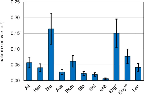
4.2 Internal balance
Results of the internal ablation calculations show that the mean contribution over 1989–2014 varies from glacier to glacier (Fig. 7). The highest values are found for Ni-gardsbreen and Engabreen),−0.16 and−0.15 m w.e. a−1, respectively. This is due to large amounts of precipitation combined with a large elevation range. All other glaciers
5
have small internal ablation rates of 0.01–0.06 m w.e. a−1, mainly due to small eleva-tion differences or small precipitation volumes. All values were calculated for a com-mon period (1989–2014) to compare the absolute contribution between the glaciers. For Engabreen the period was divided into two, before and after the subglacial wa-ter intakes constructed in 1993 when much of the sub-glacial run-offwas being
cap-10
tured by the hydropower diversion tunnel. As a result, according to the calculations, the annual contribution from internal ablation decreased from 0.15 to 0.08 m w.e. a−1. The contribution of internal and basal melt varies from year to year due to varying meteorological conditions. For example, at Nigardsbreen, the average annual inter-nal balance over 1989–2013 was calculated to be−0.16±0.04 m w.e. a−1. Values for
15
individual years over 1962–2014 ranged from −0.09 to −0.24 m w.e. a−1. The mean homogenized surface summer balance is−2.05 m w.e. over 1962–2014, so this con-tribution represents an 8±3 % additional melt from what is measured at the surface. Internal ablation is a significant contribution for the long-term series of Nigardsbreen, amounting to−8.5±2.1 m w.e. for the 53 years of measurements over 1962–2014.
20
4.3 Uncertainty and comparison
The results from the uncertainty analysis (Table 4) show that largest uncertainties were associated with point measurements at maritime glaciers (above 0.20–0.25 m w.e. a−1), followed by spatial integration at glaciers with few stakes per elevation band (about 0.15–0.21 m w.e. a−1). The largest point errors were at glaciers with a large mass
25
TCD
9, 6581–6626, 2015Glaciological and geodetic mass
balance of ten long-term glaciers in
Norway
L. M. Andreassen et al.
Title Page
Abstract Introduction
Conclusions References
Tables Figures
◭ ◮
◭ ◮
Back Close
Full Screen / Esc
Printer-friendly Version
Interactive Discussion
Discussion
P
a
per
|
Discussion
P
a
per
|
Discussion
P
a
per
|
Discussion
P
a
per
|
previous year, and difficulties in maintaining the stake network, both in summer and winter season. The largest spatial integration errors were typically at the outlet glaciers with a large accumulation plateau draining ice down through a heavily crevassed ice-fall leading to the snout – making it difficult to measure at all elevations and parts of the glacier. Other glaciers and error components were small, in the range from 0.01 to
5
0.12 m w.e. a−1. Uncertainties in geodetic mass balances were largest where old maps were used (up to 0.23 m w.e. a−1), but most are in the range from 0.05–0.10 m w.e. a−1. The error in density corrections was small (0.05 m w.e. a−1). The uncertainty in internal balance was assumed to be one third of the balance: above 0.06 m w.e. a−1 for three maritime glaciers and very small for the others.
10
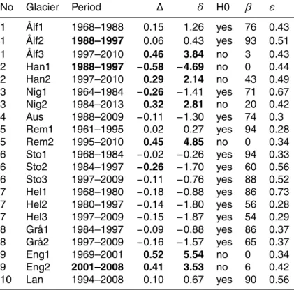
Glaciological and geodetic balances were compared for 21 periods (Table 4, Fig. 8). In this comparison, the internal balance was taken into account by subtracting it from the geodetic balance. The discrepancies and tests of the hypothesis are shown in Table 5. Good agreement (less than 0.20 m w.e. a−1) was found for 12 periods, whilst 5 periods showed discrepancies above 0.40 m w.e. a−1. The four remaining periods had
15
discrepancies between 0.26 and 0.32 m w.e. a−1. The data from the maritime glaciers (Engabreen, Nigardsbreen, Ålfotbreen, Hansebreen) deviated the most, in addition to one period for Rembesdalskåka and Storbreen. The glaciological mass balance was more positive than the geodetic for most large deviations, except for the first period of Hansebreen.
20
Uncertainty was included in the comparison in order to test the null hypothesis (H0: “the cumulative glaciological balance is not statistically different from the geodetic bal-ance”) and to check if unexplained discrepancies suggest calibration to be applied (Zemp et al., 2013). Testing at the 95 % acceptance level showed that the null hy-pothesis was rejected for seven periods: Ålfotbreen (1997–2010), Hansebreen (1988–
25
TCD
9, 6581–6626, 2015Glaciological and geodetic mass
balance of ten long-term glaciers in
Norway
L. M. Andreassen et al.
Title Page
Abstract Introduction
Conclusions References
Tables Figures
◭ ◮
◭ ◮
Back Close
Full Screen / Esc
Printer-friendly Version
Interactive Discussion
Discussion
P
a
per
|
Discussion
P
a
per
|
Discussion
P
a
per
|
Discussion
P
a
per
|
rejected. For the 12 other periods, deviations were smaller than 0.20 m w.e. a−1 and within the uncertainties at the 95 % acceptance level.
4.4 Calibration
Correcting the glaciological mass balance series with geodetic observations is recom-mended where large, relative to the uncertainties, deviations are detected between
5
glaciological and geodetic balances (Zemp et al., 2013). The deviations found between glaciological and geodetic surveys for several glaciers in our study calls for a calibration for seven of the 21 periods. Previous studies have suggested to use statistical variance analysis (Thibert and Vincent, 2009), distributed mass balance modelling (Huss et al., 2009), or by distributing equally the mean annual difference between the homogenized
10
glaciological and geodetic balance (Zemp et al., 2013). In the latter case, the difference in the annual balanceBais suggested to be fully assigned to the summer balanceBs
(Zemp et al., 2013). To calibrate our data series, we used a slightly different approach. The annual correction factor is the annual difference between the homogenized geode-tic and glaciological mass balance,∆, for each period (Table 5). This annual correction
15
factor was applied to the summer and winter balances according to their relative size. In other words, if summer and winter balances were equal, 50 % of the correction was applied to the summer balance and 50 % to the winter balance. If the absolute summer balance was twice the winter balance, 2/3 of the correction was applied to the summer balance and 1/3 to the winter balance. The reasoning behind this was that the size
20
of the error was probably related to the size of the balance. In years with thick snow, the probing to the summer surface and maintenance of the stake network were more uncertain. In years with large melt, maintenance of stake networks were more difficult and the results less accurate.
The new reanalysed glaciological series, resulting from homogenization and
calibra-25
TCD
9, 6581–6626, 2015Glaciological and geodetic mass
balance of ten long-term glaciers in
Norway
L. M. Andreassen et al.
Title Page
Abstract Introduction
Conclusions References
Tables Figures
◭ ◮
◭ ◮
Back Close
Full Screen / Esc
Printer-friendly Version
Interactive Discussion
Discussion
P
a
per
|
Discussion
P
a
per
|
Discussion
P
a
per
|
Discussion
P
a
per
|
glaciers. The major changes in cumulative balances up to and including year 2013 are (the part of reduction due to calibration is in parenthesis):
1. Engabreen reduced by 20.8 (19.3) m w.e. since 1970.
2. Nigardsbreen reduced by 14.8 (9.4) m w.e. since 1962.
3. Ålfotbreen reduced by 7.5 (5.9) m w.e. since 1963.
5
4. Rembesdalskåka reduced by 5.9 (6.8) m w.e. since 1963.
5. Austdalsbreen reduced by 3.6 m w.e. since 1988.
Austdalsbreen was not calibrated, the reduction is only due to the homogenization. At Rembesdalskåka the homogenization resulted in more positive balance, thus the calibrated part is larger than the total reduction.
10
Others glaciers had small or no change (within ±1.0 m w.e.). The new reanalysed series show a much more consistent signal then the original data (Fig. 8). The previ-ously reported difference of the cumulative balances of the maritime and continental glaciers are still present, but much less pronounced. Six glaciers have a large mass loss (cumulative balance between−14 and −22 m w.e.) and four glaciers are nearly in
15
balance (cumulative balance within±4 m w.e.). Original data showed a marked surplus for three glaciers (up to 21 m w.e.). A period of surplus is still visible in the data, but now mainly as a transient surplus for the period 1989–1995. The cumulative results further highlight the marked loss of mass during the period after 2000 for all glaciers.
5 Discussion
20
5.1 Calibration
TCD
9, 6581–6626, 2015Glaciological and geodetic mass
balance of ten long-term glaciers in
Norway
L. M. Andreassen et al.
Title Page
Abstract Introduction
Conclusions References
Tables Figures
◭ ◮
◭ ◮
Back Close
Full Screen / Esc
Printer-friendly Version
Interactive Discussion
Discussion
P
a
per
|
Discussion
P
a
per
|
Discussion
P
a
per
|
Discussion
P
a
per
|
subtracting it from the geodetic mass balance before comparing it with the glaciologi-cal. This was done to ensure that the glaciological balance was still the surface mass balance, which is what we measure for all glaciers. The amount of calibrating thus depends also on how much internal melt we estimate. The internal ablation rates cal-culated for these two maritime glaciers with a large elevation range was significant
5
and represented a marked difference between the glaciological and geodetic method. For the 49 years compared for Nigardsbreen, internal ablation amounted to nearly
−8 m w.e. according to our calculations. Oerlemans (2013) estimated an even higher
dissipative melt for Nigardsbreen of−0.23 m w.e. a−1, using this value would give more than −11 m w.e. resulting from the internal balance over the 49 years. Although both
10
values must be considered only an estimate, it points to how sensitive cumulative se-ries are both to systematic biases and to generic differences between the methods. For Engabreen, almost all the change in cumulative values is due to the calibration of the two geodetic periods and the amount of internal ablation controls the amount of calibra-tion. A higher estimate of internal ablation for this glacier would lead to a smaller deficit
15
between the methods and thus a smaller reduction in the mass surplus of the glacio-logical series. Thus, carefulness must be used when interpreting cumulative curves, in particular for glaciers located in high-precipitation regions spanning a large elevation range, such as Engabreen and Nigardsbreen.
5.2 Implications and outlook
20
The reanalysis processes has altered seasonal, annual and cumulative as well as ELA and AAR values for many of the years for the 10 glaciers presented here. For most glaciers the discrepancy between the “original” glaciological series as published in the series “Glaciolocical investigations in Norway” (e.g. Kjøllmoen et al., 2011) are small, but for others results significantly differed. We plan to keep the series “original”,
“ho-25
TCD
9, 6581–6626, 2015Glaciological and geodetic mass
balance of ten long-term glaciers in
Norway
L. M. Andreassen et al.
Title Page
Abstract Introduction
Conclusions References
Tables Figures
◭ ◮
◭ ◮
Back Close
Full Screen / Esc
Printer-friendly Version
Interactive Discussion
Discussion
P
a
per
|
Discussion
P
a
per
|
Discussion
P
a
per
|
Discussion
P
a
per
|
has been reanalysed. The data will also be submitted to WGMS and flagged with re-mark on the reanalysis status.
The level of analysis in the homogenizing process varied between the 10 study glaciers, according to the volume and quality of detailed data and metadata. For some of the glaciers (Nigardsbreen, Engabreen, Ålfotbreen and Hansebreen) a detailed
ho-5
mogenisation process was carried out going through the data material for each year to search for inhomogenities and possible biases in the data calculations. This should also be considered applied to the other six glaciers, as well as on other glaciers not considered here that have shorter series. However, for some glaciers, e.g. Rembesdal-skåka and Storbreen, the point data and metadata used for the calculations are simply
10
not available for many of the early years, and a detailed scrutinising of the data and the recalculations is not possible.
As mentioned, at many of the glaciers a change of the observation programme was carried out after statistical analysis of the previous years’ accumulation and ablation patterns in the 1980s. This was done to reduce the amount of fieldwork and hence
re-15
duce costs and personnel resources. Glaciological mass balance programmes, based on a minimal network of long-term ablation and accumulation point measurements, is recommended to increase the observational network once every decade in order to reassess the spatial pattern of mass balance (Zemp et al., 2013). The results re-vealed here may call for an increased observation network on the glaciers with largest
20
deficits if resources are available. Moreover, further research is needed to explain the discrepancy between glaciological and geodetic mass balance, as well as to adjust the observational programmes in order to reduce uncertainty. Finally, the results call for continued geodetic surveys every 10 years to measure the overall changes and provide data for new reanalysis.