APPLICATION OF AN ITERATIVE METHOD AND AN EVOLUTIONARY ALGORITHM IN FUZZY OPTIMIZATION
Ricardo Coelho Silva
1*, Luiza A.P. Cant˜ao
2and Akebo Yamakami
3Received February 4, 2011 / Accepted January 28, 2012
ABSTRACT.This work develops two approaches based on the fuzzy set theory to solve a class of fuzzy mathematical optimization problems with uncertainties in the objective function and in the set of constraints. The first approach is an adaptation of an iterative method that obtains cut levels and later maximizes the membership function of fuzzy decision making using the bound search method. The second one is a meta-heuristic approach that adapts a standard genetic algorithm to use fuzzy numbers. Both approaches use a decision criterion called satisfaction level that reaches the best solution in the uncertain environment. Selected examples from the literature are presented to compare and to validate the efficiency of the methods addressed, emphasizing the fuzzy optimization problem in some import-export companies in the south of Spain.
Keywords: fuzzy numbers, cut levels, fuzzy optimization, genetic algorithms.
1 INTRODUCTION
Mathematical programming is used to solve problems that involve minimization (or maximiza-tion) of the objective function in a function domain that can be constrained or not, as described in (Bazaraaet al., 2006) and (Luenberger & Ye, 2008). The formulation of these problems needs to describe clear, certain and brief mathematical definitions both regarding the objective function and the set of constraints. This set of problems can be formalized in the following way:
min f(x)
s. to g(x)≤b x∈
(1)
*Corresponding author
1Institute of Science and Technology, Federal University of S˜ao Paulo – UNIFESP, Rua Talim, 330, 12231-280 S˜ao Jos´e dos Campos, SP, Brazil. E-mail: ricardo.coelhos@unifesp.br
2Environmental Engineering Department, S˜ao Paulo State University – UNESP, Av. Trˆes de Marc¸o, 511, 18087-180 Sorocaba, SP, Brazil. E-mail: luiza@sorocaba.unesp.br
where ∈ Rn, f: → Randg: Rk × → Rk Applications can be found in business, industrial, military and governmental areas, among others.
However, there are ambiguous and uncertain data in real-world optimization problems. In recent years, Theory of Fuzzy Sets (Zadeh, 1965) has shown great potential for modeling systems, which are non-linear, complex, ill-defined and not well understood. Fuzzy Theory has found numerous applications due to its ease of implementation, flexibility, tolerant nature to imprecise data, and ability to model non-linear behavior of arbitrary complexity. It is based on natural language and, therefore, is employed with great success in the conception, design, construction and utilization of a wide range of products and systems whose functioning is directly based on the reasoning of human beings.
The first works showing methods that solve optimization problems in fuzzy environments were described in (Tanakaet al., 1974), (Verdegay, 1982) and (Zimmermann, 1983). The approaches there developed solve fuzzy linear programming problems. The fuzzy set theory is applied in a different branch of optimization problems,i.e., the fuzzy graph theory to solve the minimum spanning tree problem, as described in (Almeida, 2006), and the shortest path problem, as de-scribed in (Hernandeset al., 2009). Few works focus in developing methods that solve nonlinear programming problems in fuzzy environments. We can highlight some papers that solve prob-lems with uncertainties in the set of constraints, as described in (Lee et al, 1999), (Silva et al, 2008), (Trappey et al, 1988) and (Xu, 1989). Other methods deal with the uncertainties present in some parameters that can be coefficients and/or decision variables, as described in (Berredoet al., 2005), (Ekelet al., 1998), (Ekel, 2002) and (Galperin & Ekel, 2005).
In this fuzzy environment, as it happens in the case of linear programming problems, a variety of fuzzy non-linear programming problems can be defined: non-linear programming problems with a fuzzy objective,i.e., with fuzzy numbers defining the costs of the objective function; non-linear programming problems with a fuzzy goal, i.e., with some fuzzy value to be attained in the objective; non-linear programming problems with fuzzy numbers defining the coefficients of the technological matrix and, finally, with a fuzzy constraint set,i.e., with a feasible set defined by fuzzy constraints. Fuzzy numbers a˜ discussed here are defined by a triangular pertinence functionμa˜(x):R → [0,1]that associates to each x ∈Ra pertinence level. In this setting, 0
expresses complete exclusion and 1 complete inclusion. Also,a˜ ∈ F(R)is commonly referred as a fuzzy set overR.
programming problem with fuzzy coefficients in the objective function and fuzzy constraints can be formalized in the following form:
min f(˜a;x)
s. to g(x)≤f b x∈
(2)
where f: F(Rn)×→ F(R)andg:Rk×→Rk. The parametera˜ ∈ R(Rn)represents a
vector of fuzzy numbers and≤f represents the uncertainties in the constraints.
A defuzzification method, based on the first Yager’s index, is used to obtain a real number from the fuzzy objective value. Although the fuzzification of the problem data allows the decision maker to handle its uncertainties, a real (crisp) answer is desirable and easier to interpret and implement. This defuzzification process is denoted byD f(·).
Due to the increasing interest in augmentation of fuzzy systems with learning and adaptation capabilities we find works that join it with some soft computing techniques. In (Cord ´onet al., 2004), a brief introduction to models and applications of genetic fuzzy systems are presented. In addition, this work includes some of the key references about this topic. In (Coello, 2002), we can find a survey of state of the art theoretical and numerical techniques, which are used in some genetic algorithms to deal with constraint-handling optimization problems. The genetic algorithms are also used to solve multi-objective optimization problems and a hybrid approach, combining fuzzy logic and genetic algorithm, is proposed in (Sakawa, 2002).
This work is divided as follows. Section 2 introduces the adaptations of an iterative method that uses two phases to solve mathematical programming problems with fuzzy parameters in the objective function and uncertainties in the set of constraints; Section 3 introduces an adaptation of a genetic algorithm for the proposed fuzzy problems in this work; Section 4 presents a satisfaction level which tries to establish a tradeoff between α-cut level and the solution of the objective function; Section 5 presents numerical simulations for selected problems and an analysis of the obtained results. Finally, concluding remarks are found in Section 6.
2 ITERATIVE METHOD
The proposed method in this section can be used to solve non-linear programming problems with uncertainties both in the objective function and in the set of constraints. It is an adaptation of the so-called Two-Phase Method, developed to solve problems with uncertainties in the set of constraints. It is described in (Silvaet al., 2007), which adapts classic methods that solve classic mathematical programming problems. Optimality conditions described in (Cant ˜ao, 2003) were introduced into this modified method in order to solve non-linear programming problems with fuzzy parameters in the objective function.
restrictions. Therefore if we denote each constraint as gi(x), the problem at hand can be
ex-pressed as
min f(˜a;x)
s. to gi(x)≤f bi i ∈ I x∈
(3)
where the membership functions
μi:Rn→ [0,1], i ∈I
of the fuzzy constraints should be determined by the decision maker. It is patent that each mem-bership function will give the memmem-bership (satisfaction) degree with which anyx∈Rn accom-plishes the corresponding fuzzy constraint on which it is defined. This degree is equal to 1 when the constraint is perfectly accomplished (no violation), and decreases to zero according to greater violations. Finally, for non-admissible violations the accomplishment degree will equal to zero in all the cases. The violation that is related in the satisfaction degree is defined bydi for each
con-strainti. In the linear case (and formally also in the non-linear one), these membership functions can be formulated as follows
μi(x)=
1 gi(x) <bi
1− gi(x)−bi
di bi ≤gi(x)≤bi+di
0 gi(x) >bi+di
In order to solve this problem in a two-phase method, first let us define for each fuzzy constraint,
i ∈I
Xi =
x∈Rn|gi(x)≤f bi, x∈ .
IfX = ∩i∈IXi then the former fuzzy nonlinear problem can be addressed in a compact form as
minf(˜a;x)|x∈ X .
Note that∀α∈ [0,1], anα-cut of the fuzzy constraint set will be the classical set
X(α)=x∈Rn|μX(x) > α .
where∀x∈Rn,
μX(x)=inf[μi(x)], i∈ I.
Hence anα-cut of thei-th constraint will be denoted byXi(α). Therefore, if∀α∈ [0,1],
S(α)=x∈Rn|f(˜a;x)=min f(˜a;y),y∈ X(α)
the fuzzy solution of the problem will be the fuzzy set defined by the following membership function
S(x)=
(
sup{α:x∈S(α)} x∈ ∩αS(α)
S(x)represents the biggest pertinence level (than the sup) for a givenα-cut, that minimizes the fuzzy problem.
Provided that∀α∈ [0,1],
X(α)=\ i∈I
x∈Rn|gi(x)≤ri(α), x∈
withr(α)=bi+di(1−α), the operative solution to the former problem can be found,α-cut by α-cut, by means of the following auxiliary parametric nonlinear programming model
min f(˜a;x)
s. to gi(x)≤bi +di(1−α) i ∈I α∈ [0,1], x∈
(4)
It is easy to see that Problem (4) can have two possibilities: (i) it has a new decision variable
α∈ [0,1], which helps to transform a fuzzy optimization problem into a classical one; or (ii) it has a parameter because we can discretizeαbetween 0 and 1.
It is clear that one of them is chosen the first phase of this method ends at the start of the second one. In this case we will choose the parameter approach.
In the second phase we solve the parametric nonlinear programming problem determined in the previous step to each one of the differentαvalues using conventional nonlinear programming techniques. We must find solutions of Problem (4) to each α that satisfy the Karush-Kuhn-Tucker’s necessary and sufficient optimality conditions. One of the conventional techniques is to write the Lagrange function that is a transformation of Problem (1) as an unconstrained mathematical problem in the following form:
L(˜a;x, η)= f(˜a;x)+ηt gi(x)−bi −di(1−α)
, ∀x∈ (5)
whereηis the Lagrange multiplier for the inequality. The obtained results, for differentα val-ues, generate a set of solutions and then we use the Representation Theorem to integrate all of these particularα-solutions. Note that the computational complexity depends on the optimiza-tion technique, such as Barrier and Penalty methods, chosen to solve the transformed problem. In addition, some real problems can be harder to solve them by using classical optimization techniques. So we decide to join the approach with a new decision variable and a genetic algo-rithm. The genetic algorithm will be presented in the next section and then these two approaches will be compared in the Section 5.
3 GENETIC ALGORITHM
Genetic algorithms have obtained considerable success during the last decades when applied to a wide range of problems, such as optimal control, transport, scheduling problems among oth-ers. The implementation of the algorithm here proposed was based on (Liu & Iwamura, 1998a; 1998b), with some modifications. The adapted genetic algorithm in this work uses only basic evolutionary strategies, namely: selection process, crossover operation and mutation operation. Later on we will describe a pseudo-code of this algorithm.
3.1 Structure representation
The approach used to represent a solution is the floating point implementation, where each chro-mosome has the same length as the solution vector. Here we use a vectorVi = xi1,x2i, . . . ,xin
, withi =1,2, . . . ,popsizeas a chromosome to represent a possible solution to the optimization problem, wherenis the dimension.
3.2 Initialization process
We define an integerpopsize = 10·n as the number of chromosomes and initializepopsize
randomly for each chromosome. We choose an interior point to initialize the population, denoted byV0, and selectpopsizeindividuals randomly in a given neighborhood of this point. We define a large positive number Ŵwhich is a step to be taken in a randomly selected direction. This numberŴis used not only for the initialization process but also for the mutation operation. We randomly select a direction di ∈ Rpopsi ze and define a chromosomeVi = V0+Ŵ·di. This chromosome is added to the initial population if it represents a feasible solution; otherwise, we randomly select another Ŵin the interval [0, Ŵ]until V0+Ŵ·di is feasible. We repeat this processpopsizetimes and producepopsizeinitial feasible solutionsV1,V2, . . . ,Vpopsi ze.
3.3 Fitness value
The fitness function evaluates the quality of each individual in the population at each iteration. The fitness of a given individual can be evaluated in several ways. Some forms of computing the fitness values can be found in (Goldberg, 1989) and (Michalewics, 1996). In this work, the value of the objective function was chosen as the fitness value for each individual. Since this value is a fuzzy number, then we apply a defuzzification method to find a classic number which best represents the fitness distribution that is Yager’s first index. In (Klir & Folger, 1998) and (Pedrycs & Gomide, 1998), other defuzzification methods are presented.
3.4 Evaluation function
good to bad (best fitness values for the worse chromosomes). Leta ∈(0,1)be a parameter in the genetic system. We can define the so-called rank-based evaluation function as follows:
eval(Vi)=a(1−a)i−1, i =1,2, . . . ,popsize.
We mention thati =1 means the best individual,i =popsizethe worst individual, and
popsizeX
i=0
eval(Vi)≈1.
3.5 Selection process
The selection process is based on spinning the roulette wheelpopsizetimes, each time selecting a single chromosome for an auxiliary population in the following way:
1. Calculate the cumulative probabilityqifor each individualVi,
q0 = 0,
qi = i
X
j=1
eval(Vj), i =1,2, . . . ,popsize;
2. Generate a random real numberrin0,qpopsi ze
;
3. Select theith individualVi,(1≤i ≤popsize)such thatq
i−1<r ≤qi;
4. Repeat steps 2 and 3popsizetimes and obtainpopsizeindividuals.
3.6 Crossover operator
We define a parameter Pc to determine the probability of crossover. This probability gives us
the expected numberPc·popsizeof chromosomes which undergo the operation. We denote the
selected parents asF1,F2, . . .and divide them in pairs. At first, we generate a random number
cfrom the open interval(0,1), then we produce two childrenC1 andC2using the crossover operator as follows:
C1 = c∗F1+(1−c)∗F2,
C2 = c∗F1+(1−c)∗F2.
3.7 Mutation operator
A parameter Pmis defined as the probability of mutation. This probability gives us the expected
number of Pm·popsizeof chromosomes which undergo the mutation operations. For each
se-lected parent, denoted byVi =(x1, . . . ,xn)we choose a mutation directiondi ∈Rnrandomly.
If Mi = Vi +Ŵ·di is not feasible we setŴ as a random number between 0 andŴuntil it is feasible. If the above process fails to find a feasible solution in a predetermined number of iterations, we setŴ=0.
3.8 Pseudo-code for the genetic algorithm
Following selection, crossover and mutation, the new population is ready and we start a new iteration. The genetic algorithm will terminate after a given number of cyclic repetitions of the above steps. The pseudo-code of the genetic algorithm has the following form:
Algorithm 1 – adapted genetic algorithm
Input: Parameterpopsize,PcandPm
Output: The best individual in all generations.
Step 01: Initializepopsizeindividuals;
Step 02: Check feasibility of each individual;
WHILEnumber of generations is less than MAX GENERATIONDO Step 03: Compute the fitness of each individual;
Step 04: Order the population, compute evaluation value;
Step 05: Perform the selection process;
Step 06: Use the crossover operator and check feasibility;
Step 07: Use the mutation operator and check feasibility;
Step 08: Update the population for the next generation;
END
4 SATISFACTION LEVEL
We define a satisfaction level representing the compromise between the objective function value and the satisfaction level of the pertinence function associated to the fuzzy inequalities. This level determines the lower bound for the membership value of the admissible solutions.
The solution of the Problem (4) belongs to the bounded interval forα∈ [0,1]that generates the upper and lower values of the form
˜
m = f(˜a; ˜x(0)) = minx∈X(0) f(˜a; ˜x) ˜
M = f(˜a; ˜x(1)) = minx∈X(1) f(˜a; ˜x),
(6)
where X(0)and X(1)are the cut levels forαequal to 0 and 1, respectively. Numbersm˜ and
˜
present on the objective function (Kaufmann et al, 1991). In a fuzzy optimization problem we can establish the fuzzy goal as follows:
μG˜(x) =
˜ m
f(˜a; ˜x). (7)
As expected, this fuzzy goal shows that when f reaches its infimum m the full membership
(μG˜ =1)is obtained; as f increasesμG˜ approaches the null membership(μG˜ =0)boundary.
Clearly, the upper and lower limits of the fuzzy goal are given by
μuG = 1
μlG = D f
˜ m ˜ M
, (8)
whereD f(·)is Yager’s first index defuzzification method, as previously mentioned. However, if the objective is to maximize or the lower and upper values are negative, we can invert the division of the Equation (7), and then, the equation of the lower limit of the fuzzy goal is defined as
μlG = D f
˜ m ˜ M
.
The minimum satisfaction level is determined by the quotient between the solution of the problem with totally violated constraints and the solution with totally satisfied constraints, see (Silvaet al., 2005) and (Silvaet al., 2006). This quotient is a fuzzy number that is determined by a fuzzy relation. The chosen defuzzification method is the modal value to determine the inferior bound.
The iterative method then performs a search in the intervalμlG(x), μuG(x)to find the optimal
α-level according to (Bellman & Zadeh, 1970). The genetic algorithm uses the inferiorα-level to determine when a solution is feasible or not.
5 NUMERICAL EXPERIMENTS
The problems to evaluate the developed methods are presented in Subsection 5.1. There are three hypothetic formulations and a fuzzy optimization problem in some import-export companies in South-east Spain. Nevertheless, they are efficient to validate the study realized.
The computational results and a comparative analysis of the classic methods and the iterative methods responses are presented in Section 5.2.
For all examples, we use the following genetic algorithm parameters:
• Crossover probability Pc=0.2;
• Mutation probabilityPm =0.1;
• Number of generations (iterations): 1000.
5.1 Formulation of the problem
In this paper we present some theoretical and real-world problems found in the literature in order to validate the proposed algorithms. We simulate four nonlinear programming problems: three theoretical problems and one real-world problem in some import-export companies in South-east Spain. All problemas have uncertainties on the parameters of the objective function.
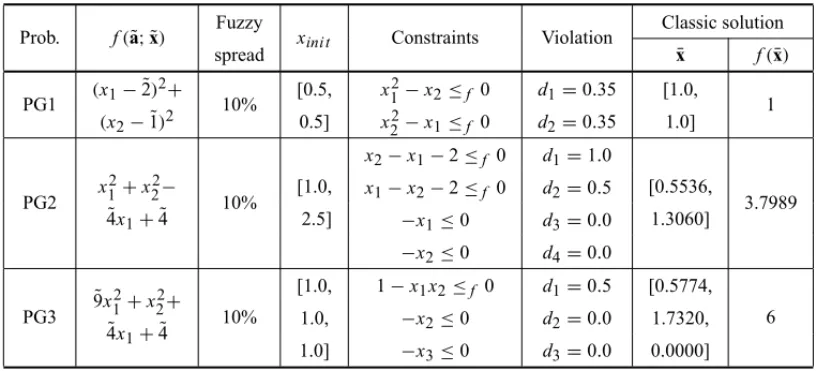
5.1.1 Theoretic tests problems
The problems with inequality constraints, described in Table 1, were taken from (Schittkowski, 1987). Uncertainties were inserted into the parameters of the objective functions in the form of a 10% variation in the modal value. The maximum violation of each constraint of the problem is a hypothetical value and it was inserted to suppose a set of well-known constraints. The optimal solutions to the problems without uncertainties are presented in the columnsx¯and f(¯x)
of Table 1.
Table 1– Theoretical problems consisting only of inequality constraints.
Prob. f(˜a; ˜x) Fuzzy xini t Constraints Violation
Classic solution
spread x¯ f(x)¯
PG1 (x1− ˜2) 2+
10% [0.5, x
2
1−x2≤f 0 d1=0.35 [1.0,
1 (x2− ˜1)2 0.5] x22−x1≤f 0 d2=0.35 1.0]
PG2 x
2 1+x22−
10% [1.0,
x2−x1−2≤f 0 d1=1.0
[0.5536,
3.7989 ˜
4x1+ ˜4 2.5]
x1−x2−2≤f 0 d2=0.5
1.3060]
−x1≤0 d3=0.0
−x2≤0 d4=0.0
PG3 ˜
9x12+x22+
10%
[1.0, 1−x1x2≤f 0 d1=0.5 [0.5774, 6 ˜
4x1+ ˜4
1.0, −x2≤0 d2=0.0 1.7320,
1.0] −x3≤0 d3=0.0 0.0000]
5.1.2 Real-world problem
Table 2– Problem in some import-export companies in the south of Spain.
Prob. f(˜a; ˜x) xini t Constraints Violation
Classic solution
¯
x f(¯x)
PCSS 23.0gx1+32.0gx2− [0.0,
10x1+6x2≤f 2500 d1=0.0
[84.8810,
5686.9 g
0.04x1−0.03gx2 0.0]
5x1+10x2≤f 2000 d2=64.0
145.5800] 7x1+10x2≤f 2050 d3=74.0
5.2 Results and analysis
In Tables 1 and 2, we presented the problem formulations and their classical solutions. In this subsection we show the results obtained for the problems in sub-section 5.1 by the iterative method presented in section 2 and by the genetic algorithm introduced in 3.
Tables 3 and 5 refer to the results obtained on the first-phase of the method from Section 2 in two forms: (i) completely satisfied restrictions, includingα=1 and, (ii) restrictions completely violated(α =0). Tables 4 and 6 bring the results from second-phase, Sections 2 and 3. The column corresponding to f(˜a;x)shows a 3-vector: first and third components are the spread, while second component is the modal value. Columnμpresents the comparison between the
α-cut level and the solution of the objective function as discussed on Section 4. The closer μ
is from 1 (one), the better the compatibility among the pertinences of both the objective and the restriction set.
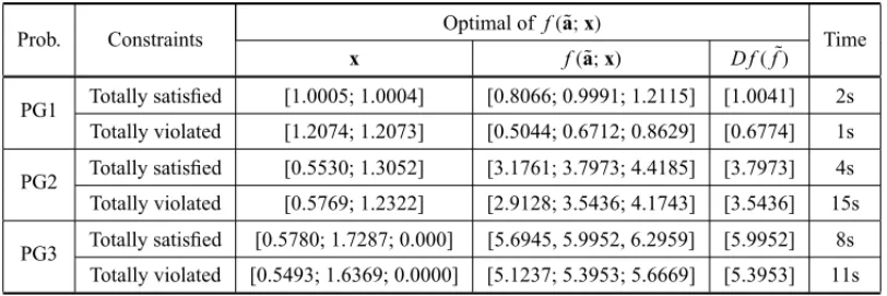
Table 3– Maximum and minimum levels of tolerance for the set of constraints.
Prob. Constraints Optimal off(˜a;x) Time
x f(˜a;x) D f(f˜)
PG1 Totally satisfied [1.0005; 1.0004] [0.8066; 0.9991; 1.2115] [1.0041] 2s Totally violated [1.2074; 1.2073] [0.5044; 0.6712; 0.8629] [0.6774] 1s
PG2 Totally satisfied [0.5530; 1.3052] [3.1761; 3.7973; 4.4185] [3.7973] 4s Totally violated [0.5769; 1.2322] [2.9128; 3.5436; 4.1743] [3.5436] 15s
PG3 Totally satisfied [0.5780; 1.7287; 0.000] [5.6945, 5.9952, 6.2959] [5.9952] 8s Totally violated [0.5493; 1.6369; 0.0000] [5.1237; 5.3953; 5.6669] [5.3953] 11s
By examining the results presented in Table 3, we can calculate the minimum satisfaction level to each problem in Table 1 of fuzzy mathematical programming problems with uncertainties in objective function and in set of constants shown in this work.
Table 4– Results using iterative method and pure genetic algorithm.
Prob. Algorithm Optimal of f(a;˜ x) Time
x f(˜a;x) D f(f˜) μ=α
PG1 Section 2 [1.058; 1.058] [0.7091; 0.8908; 1.0974] [0.8970] 0.7575 4s Section 3 [1.0608; 1.0454] [0.5385; 0.8842; 1.3189] [0.9071] 0.7591 12s
PG2 Section 2 [0.5547; 1.3015] [3.1607; 3.7826; 4.4045] [3.7826] 0.9361 11s Section 3 [0.52202; 1.2306] [2.9113; 3.6988; 4.4863] [3.6988] 0.9580 11s
PG3 Section 2 [0.5764; 1.7191; 0.000] [5.6464; 5.9454; 6.2444] [5.9454] 0.9169 5s Section 3 [0.5559; 1.7345; 0.0827] [5.2659; 5.8510; 6.4361] [5.8663] 0.9197 8s
genetic algorithm had better defuzzification value and satisfaction level. In PG3, the iterative method was faster, but the genetic obtained better defuzzification value and satisfactions level. We obtain satisfaction levels higher than 75% for all the problems. The good quality of the obtained solution is confirmed by the fact that the defuzzified values of the objective function for each problem are lower than those of the classic solution.
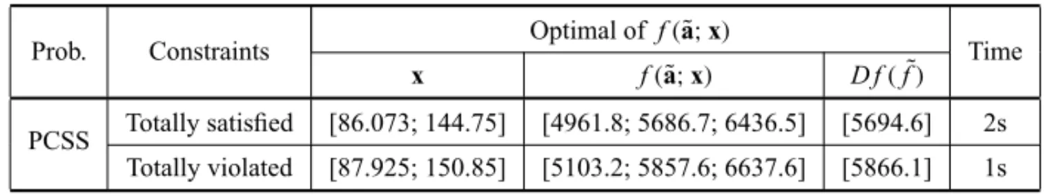
Table 5 depicts the optimal solutions of the real-world problem in two forms: (i) totally satis-fied constraints; and (ii) totally violated constraints. Table 5 shows the results for Problem (4) imposingα=1, for case (i), andα=0, for case (ii).
Table 5– Maximum and minimum levels of tolerance for the set of constraints.
Prob. Constraints Optimal of f(˜a;x) Time
x f(˜a;x) D f(f˜)
PCSS Totally satisfied [86.073; 144.75] [4961.8; 5686.7; 6436.5] [5694.6] 2s Totally violated [87.925; 150.85] [5103.2; 5857.6; 6637.6] [5866.1] 1s
In Table 6, we explore the results for the real-world problem. Note that the iterative method obtained a satisfaction level near 100%. However, the genetic algorithm presented the best fuzzy result and defuzzification value with lower processing time.
Table 6– Result to the problem with triangular fuzzy numbers.
Prob. Algorithm Optimal of f(a;˜ x) Time
x f(˜a;x) D f(f˜) μ=α
PCSS Section 2 [84.813; 145.63] [4962.2; 5686.9; 6436.5] [5695.2] 0.9992 6s Section 3 [82.7938; 147.231] [4965.9; 5691.2; 6441.3] [5699.4] 0.9172 2s
main objective to be reached. In this case, the genetic algorithm was faster than the iterative method.
6 CONCLUSION
The first method described in this work transforms the fuzzy non-linear programming problem in a parametric non-linear programming problem. The parameter is in the unit interval and we obtain the optimal solution of each discretized value of the parameter. The evolutionary algo-rithm described previously presents the basic steps of a standard genetic algoalgo-rithm but there is a difference regarding the objective function value of the non-linear programming problem with fuzzy parameters. The satisfaction level was described in this work to determine a compromise between the fuzzy goal of the objective function and the permitted violation level of each one of the membership function of the constraints.
We developed an interactive method and a genetic algorithm to solve mathematical programming problems with uncertainties in objective function and in set of constraints. The iterative method uses the differentiation from the objective function that presented good responses to proposed problems. The obtained results were better than the classic results found in the literature. The genetic algorithm presented good responses to the same problems. However, they presented a satisfaction level smaller than 100%,i.e., the optimum solution violates one or more constraints of the problem.
REFERENCES
[1] ALMEIDATA, YAMAKAMIA & TAKAHASHIMT. 2006. Sistema imunol´ogico artificial para re-solver o problema da ´arvore geradora m´ınima com parˆametros fuzzy.Pesquisa Operacional,27(1): 131–154.
[2] BAZARRAMS, SHERALIHD & SHETTYCM. 2006.Nonlinear Programming – Theory and Algo-rithms. 3rded., John Wiley & Sons, New York.
[3] BELLMANRE & ZADEHLA. 1970. Decision-making in a fuzzy environment,Management Science, 17(4): B141–B164.
[4] BERREDORC, EKELPY & PALHARESRM. 2005. Fuzzy preference relations in models of decision making.Nonlinear Analysis,63: e735–e741.
[5] CANTAO˜ LAP. 2003. Programac¸˜ao n˜ao-linear com parˆametros fuzzy. Tese de doutorado. FEEC – Unicamp, Campinas, Marc¸o.
[6] COELLOCAC. 2002. Theoretical and numerical constraint-handling techniques used with evolution-ary algorithms: a survey of state of the art.Computer Methods and Applied Mechanics and Engineer-ing,191: 1245–1287.
[7] CORDON´ O, GOMIDEF, HERRERAF, HOFFMANNF & MAGDALENAL. 2004. Ten years of genetic fuzzy systems: current framework and new trends.Fuzzy Sets and Systems,141(1): 5–31.
[9] EKEL PY. 2002. Fuzzy sets and models of decision making.International Journal Computers & Mathematics with Applications,44: 863–875.
[10] EKELPY, PEDRICZW & SCHINZINGERR. 1998. A general approach to solving a wide class of fuzzy optimization problems.Fuzzy Sets and systems,97: 46–66.
[11] GALPERINEA & EKELPY. 2005. Synthetic realization approach to fuzzy global optimization via gamma algorithm.Mathematical and Computer Modelling,41: 1457–1468.
[12] GOLDBERG DE. 1989. Genetic Algorithms in Search, Optimization, and Machine Learning, Addison-Wesley, Reading.
[13] HERNANDESF, BERTONL & CASTANHO MJP. 2009. O problema de caminho m´ınimo com in-certezas e restric¸ ˜oes de tempo.Pesquisa Operacional,29(2): 471–488.
[14] JIMENEZ´ F, CADENASJM, S ´ANCHEZG, G ´OMEZ-SKARMETAAF & VERDEGAYJL. 2006. Multi-objective evolutionary computation and fuzzy optimization.International Journal of Approximate Reasoning,43(1): 59–75.
[15] KAUFMANNA & GUPTAMM. 1991.Introduction to Fuzzy Arithmetic: Theory and Applications. Van Nostrand Reinhold.
[16] KLIRGJ & FOLGERTA. 1998.Fuzzy Sets, Uncertainty and Information, Prentice Hall, New York. [17] LEEYH, YANGBH & MOONKS. 1999. An economic machining process model using fuzzy
non-linear programming and neural network.International Journal of Production Research,37(4): 835– 847.
[18] LIUB & IWAMURAK. 1998a. Chance constrained programming with fuzzy parameters.Fuzzy Sets and Systems,94: 227–237.
[19] LIUB & IWAMURAK. 1998b. A note on chance constrained programming with fuzzy coefficients.
Fuzzy Sets and Systems,100: 229–233.
[20] LUENBERGERDG & YEY. 2008.Linear and Nonlinear Programming. 3rded., Addison-Wesley,
Massachusetts.
[21] MICHALEWICS Z. 1996. Genetic Algorithms + Data Structure = Evolution Programs. 3rd ed., Springer, New York.
[22] PEDRYCSW & GOMIDEF. 1998.An Introduction of Fuzzy Sets – Analysis and Design. A Bardford Book.
[23] SAKAWAM. 2002.Genetic algorithms and fuzzy multi-objective optimization. Kluwer Academic Publishers.
[24] SCHITTKOWSKIK. 1987.More Test Examples for Nonlinear Programming Codes. Springer-Verlag. [25] SILVARC, CANTAO˜ LAP & YAMAKAMIA. 2005. Meta-heuristic to mathematical programming
problems with uncertainties. In:II International Conference on Machine Intelligence, Tozeur-TN. [26] SILVARC, CANTAO˜ LAP & YAMAKAMIA. 2006. Adaptation of iterative methods to solve fuzzy
mathematical programming problems.Transactions on Engineering, Computing and Technology,14: 330–335.
[28] SILVARC, VERDEGAY JL & YAMAKAMI A. 2007. Two-phase method to solve fuzzy quadratic programming problems. In: 2007 IEEE International Conference on Fuzzy Systems, London-UK, 1–6.
[29] TANAKAH, OKUDAT & ASAIK. 1974. On fuzzy-mathematical programming.Journal of Cyber-netics,3(4): 37–46.
[30] TRAPPEYJFC, LIUCR & CHANGTC. 1988. Fuzzy non-linear programming: theory and applica-tion in manufacturing.International Journal of Production Research,26(5): 975–985.
[31] VERDEGAYJL. 1982. Fuzzy mathematical programming. In: Fuzzy Information and Decision Proc-sses, Gupta MM & Sanches E (eds.). North-Holland Publishing Company, Amsterdan.
[32] XUC. 1989. Fuzzy optimization of structures by the two-phase method.Computers & Structures, 31(4): 575–580.
[33] ZADEHLA. 1965. Fuzzy sets.Information and Control,8: 338–353.