Understanding the Spatial Scale of Genetic
Connectivity at Sea: Unique Insights from a
Land Fish and a Meta-Analysis
Georgina M. Cooke1,2*, Timothy E. Schlub3, William B. Sherwin1, Terry J. Ord1
1Evolution and Ecology Research Centre, School of Biological, Earth and Environmental Sciences, University of New South Wales, Kensington 2052 NSW, Australia,2The Australian Museum, Australian Museum Research Institute, Ichthyology, 6 College Street, Sydney NSW 2010, Australia,3Sydney School of Public Health, Sydney Medical School, University of Sydney, 2006 NSW, Australia
Abstract
Quantifying the spatial scale of population connectivity is important for understanding the evolutionary potential of ecologically divergent populations and for designing conservation strategies to preserve those populations. For marine organisms like fish, the spatial scale of connectivity is generally set by a pelagic larval phase. This has complicated past estimates of connectivity because detailed information on larval movements are difficult to obtain. Genetic approaches provide a tractable alternative and have the added benefit of estimat-ing directly the reproductive isolation of populations. In this study, we leveraged empirical estimates of genetic differentiation among populations with simulations and a meta-analysis to provide a general estimate of the spatial scale of genetic connectivity in marine environ-ments. We used neutral genetic markers to first quantify the genetic differentiation of eco-logically-isolated adult populations of a land dwelling fish, the Pacific leaping blenny (Alticus arnoldorum), where marine larval dispersal is the only probable means of connectivity among populations. We then compared these estimates to simulations of a range of marine dispersal scenarios and to collatedFSTand distance data from the literature for marine fish
across diverse spatial scales. We found genetic connectivity at sea was extensive among marine populations and in the case ofA.arnoldorum, apparently little affected by the pres-ence of ecological barriers. We estimated that ~5000 km (with broad confidpres-ence intervals ranging from 810–11,692 km) was the spatial scale at which evolutionarily meaningful barriers to gene flow start to occur at sea, although substantially shorter distances are also possible for some taxa. In general, however, such a large estimate of connectivity has important implications for the evolutionary and conservation potential of many marine fish communities.
a11111
OPEN ACCESS
Citation:Cooke GM, Schlub TE, Sherwin WB, Ord TJ (2016) Understanding the Spatial Scale of Genetic Connectivity at Sea: Unique Insights from a Land Fish and a Meta-Analysis. PLoS ONE 11(5): e0150991. doi:10.1371/journal.pone.0150991
Editor:Zhengfeng Wang, Chinese Academy of Sciences, CHINA
Received:August 27, 2015
Accepted:February 21, 2016
Published:May 19, 2016
Copyright:© 2016 Cooke et al. This is an open access article distributed under the terms of the
Creative Commons Attribution License, which permits unrestricted use, distribution, and reproduction in any medium, provided the original author and source are credited.
Data Availability Statement:All data from this publication have been archived in the Dryad Digital Repository (doi:10.5061/dryad.v63g0) and Genbank (KU922092-KU922117).
Funding:This work was supported by Evolution and Ecology Research Centre start-up funds, a University of New South Wales Science Faculty Research Grant and Australian Research Council major grant to TJO.
Introduction
Genetic exchange among individuals and between populations—i.e. genetic connectivity—is important for the evolutionary dynamics of species across all spatial and temporal scales, from a local to regional level and from thousands to millions of years. Indeed, there has been enor-mous interest in estimating gene flow across space and time and this information has been used to understand biological and evolutionary processes like adaptation, biogeographic his-tory and speciation [1]. In addition, estimations of gene flow are being used to improve the design and implementation of management strategies that maximise genetic fitness among threatened populations through the appropriate spatial placement of reserves or wildlife corri-dors [2]. However, for organisms in which dispersal is characterized by small gametes or off-spring—e.g. marine fish with pelagic larvae—accurate predictions of the degree to which populations are impacted by dispersal and subsequent connectivity (also known as‘ demo-graphic connectivity’) have been difficult to make. This is partly because the nature of marine ecosystems often precludes the direct measure of the number and type of individuals moving or interacting among populations (also known as demographic connectivity e.g. through tag-ging and mark-re-capture [3,4]). Indeed, for many fish species, the spatial scale of connectivity is set by pelagic larvae that may be dispersed by highly advective ocean currents for several days to weeks before settlement, which might then be followed by either a sedentary or migra-tory adult phase [5–9]. This means that populations of marine fish appear to have high connec-tivity across very large spatial scales often upwards of 300 km [9–12]. Yet, despite the apparent capacity for high genetic exchange at sea, the behaviour of larval fish can also limit dispersal. In particular, larvae are capable of highly directional swimming that can minimize the influence of mean ambient currents [13] and can result in self-recruitment to natal habitats despite oce-anic currents. This in turn reduces connectivity to much smaller spatial scales [13–16]. Conse-quently, predicting the magnitude and geographic scale of connectivity of fish in the marine environment has been a notoriously difficult task.
Given this difficulty in measuring marine connectivity, indirect methods such as the genetic estimation of population structure and gene flow have been employed [9]. Because differentia-tion of neutral genes among populadifferentia-tions is dependent on gene flow, differentiadifferentia-tion is expected to be affected by dispersal ability, restriction of population size and the extent of isolation and habitat connectivity. Therefore, genetic analysis of population structure using Wright’sFST ([17]; and its analogues) has been a common genetic method for estimating the spatial scale and magnitude of connectivity in the marine environment [9,18]; e.g. the relationship between pelagic larval dispersal in distance (PLD) andFST[19,20,21]. One such model is Wright’s [17] island model in which there is equal dispersal between all pairs of local populations (such equal dispersal is unlikely in most systems, but the model nevertheless provides useful predictions that can be used to benchmark data). An alternative model, known as isolation by distance (IBD; [22]), has higher dispersal between closer localities, such that closer populations will be more similar at neutral genetic markers. In other words, isolation by distance predicts that pairwise genetic divergence (FSTor alternatives) among populations will be positively corre-lated with geographic distance (e.g. [23]). As a result of the arguably more realistic“stepping stone”scenario of IBD theory, it has been a frequently utilized model in studies of marine con-nectivity [12,24,25]. Despite this, there is considerable debate surrounding the relationship between dispersal andFST[26,27], as well as the effectiveness ofFSTas a measure of genetic structure compared to its analogues (e.g. [28–31]). While many of these authors have
it continues to be one of the most valuable metrics for the quantification of genetic connectivity in marine fish and subsequent comparison among published data.
In this study we combined several complementary approaches combined with a meta-analy-sis (Fig 1;S1 Fig) to better understand and predict the spatial scale of genetic connectivity in marine fishes. First, we examined connectivity in the context of population demography and fine scale genetic structure among populations of an unusual fish, the Pacific leaping blenny
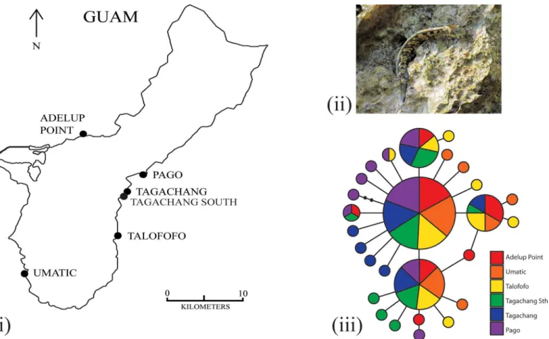
(Alticus arnoldorum) found on the Micronesian island of Guam (Fig 2i and 2ii).
Alticus arnoldorumlive their adult life out of water at high densities along the supralittoral
zone [32]. They have enhanced cutaneous respiration [33–35] and terrestrial locomotor abili-ties that allow them to move about with extreme agility on land [36]. Adult fish are highly terri-torial and are rarely seen to voluntarily return to water [32]. The fish are susceptible to
desiccation at low tides and displacement from perches by violent wave action at high tide. This results in a brief temporal window at mid-tide during which most activity is restricted (e.g. foraging) and more generally confines these land fish to the supralittoral splash zone on the island [32]. Given that suitable habitat for this fish around the coast of Guam is discontinu-ous–the rocky outcrops on which they live are interspersed by large beaches that represent a formidable barrier to these fish–adult dispersal among populations is virtually impossible. However, the larvae ofA.arnoldorumare almost certainly pelagic (settlement occurs around 28 days, Platt and Ord, unpublished), and are the most likely means by which individuals might be exchanged among populations. Because of this,A.arnoldorumprovides a good opportunity to quantify the geographic extent of connectivity among populations that results primarily from the movement of marine larvae. This can be extremely difficult to achieve in genetic studies of population structure in the marine environment that sum the results of larval and adult dispersal (for rare examples see [37–40]).
We compared our estimates of population genetic differentiation ofA.arnoldorumon Guam to genetic differentiation data from simulations that assumed a range of realistic marine dispersal scenarios for this species. The simulation used a spatial matrix of the inter-tidal zone around Guam and used various density-dependent models of dispersal. Thus, we were able to evaluate the extent to which a primarily larval-dispersed marine fish exhibited predictable or unexpected levels of population genetic differentiation.
Second, we placed these findings from the larval-dispersingA.arnoldoruminto its broadest context by obtaining a general estimate of connectivity among marine fishes (that might reflect dispersal via larvae, adults or both) using a meta-analysis ofFSTand distance data from pub-lished literature. Estimates of gene flow usingFSThave been documented by hundreds of stud-ies for an equally vast number of spatial scales and different organisms including fishes. We took advantage of this enormous resource to estimate the rate at which gene flow is curbed by distance in marine fish across all environments and spatial scales. In doing so, we generalised the extent to whichFSTincreases with distance and the magnitude of connectivity in marine fish globally.
By integrating an empirical study, simulations and a meta-analysis (Fig 1), our overarching goal was to estimate the spatial scale of genetic connectivity at sea for fish and evaluate the extent to which pelagic larval dispersal in fish impacts genetic connectivity among populations that are otherwise isolated from one another by ecological barriers to adult dispersal. To this end, we tested three possible scenarios of how the behaviour of larvae might impact genetic connectivity (Fig 3):
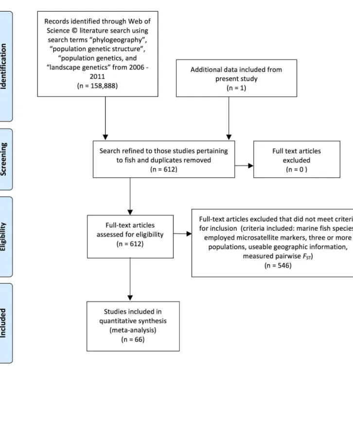
Fig 1. PRISMA 2009 Flow diagram.Depicts the selection process of studies included in the meta-analysis.
populations that are geographically close (i.e.<100km, or significantFSTbetween popula-tions around Guam). This outcome would indicate a more terrestrial mode of dispersal. Indeed, terrestrial animals such as mammals that cannot disperse in their earliest develop-mental stage generally have higher globalFSTthan larval dispersers like fish [41]. In some cases, significant genetic structure can be observed in small mammals across distances as lit-tle as<10km (e.g. [42]). Given this, the rate of IBD inA.arnoldorumshould be much higher than the median rate for marine fish collated in our meta-analysis if combined larval and adult dispersal results in high genetic connectivity in the marine environment (i.e. [9–
12]).
2. Alternatively, connectivity among populations ofA.arnoldorummight result from passive larval dispersal driven by ocean eddies and currents around Guam, followed by a sedentary adult phase (i.e., a transition from a marine to land environment where adult populations are subsequently ecologically isolated from one another). In this scenario, a Lagrangian lar-val dispersal model [43] that assumes a one month pelagic larval period similar to that ofA.
arnoldorumpredicts dispersal distances of up to 300km (~10km/day). As the circumference
of Guam falls within this distance (~150 km), there should be no significant population structure among populations ofA.arnoldorum. Instead, the globalFSTofA.arnoldorum should be similar to simulations that assume high dispersal scenarios (greater than the Fig 2. Sampling localities and haplotype network.The (i) sampling localities ofAlticus arnoldorumaround the island of Guam, site abbreviations as in
Table 1, (ii)A.arnoldorum(photo G Cooke), and (iii) results from the haplotype network based on 120 mtDNA ATPase 6 and 8 sequences. Each circle denotes a unique haplotype, the area of the circle is proportional to its frequency in the sample, and the shade of the circle represents its sampling location.
maximum distance between any two populations, i.e. 300km) with a rate of IBD inA.
arnol-dorumbeing equal to, or less than, the median rate for marine fish estimated by our
meta-analysis.
3. Finally, connectivity among populations ofA.arnoldorummight be a combination of pas-sive and active larval dispersal, followed by a sedentary adult phase (see scenario 2 above). Such a pattern could occur if natural selection is acting on a local level either before or after settlement due to ecological differences between sites (e.g., see [44]). In this situation we expect to see some genetic structure or‘chaotic genetic patchiness’in which there is small-scale, unpatterned genetic heterogeneity among local populations [45,46], which may not necessarily be correlated with distance. Here, some cohesion or active dispersal of larvae between sites may skew the relationship between geographic distance and genetic diver-gence. Furthermore, globalFSTshould be similar to or higher than simulations that assume Fig 3. Scenarios of how the behaviour of larvae might impact genetic connectivity(i) Predictions based on realistic dispersal scenarios ofAlticus arnoldorumincorporating empirical, simulated and meta-analyses results. (ii) Schematic illustrating the results fromAlticus arnoldorumcompared to the simulated and meta-analysis results.
moderate dispersal scenarios (greater than or equal to the maximum distance between any two populations), and the rate of IBD inA.arnoldorumshould be equal to, or greater than, the median rate ofFSTand distance for marine fish from our meta-analysis.
Materials and Methods
Sampling and genetic methods
This study was carried out following procedures set by the University of New South Wales Ani-mal Care and Ethics Committee in protocol #11/36b, initially approved on the 10th March 2011 and most recently reviewed on the 28th February 2013. Specimens were euthanized by first anaesthetizing fish using clove oil and then storing them under ice. No permits or approv-als were required to collect specimens on Guam, and no work was conducted on private or pro-tected land. All data from this publication have been archived in the Dryad Digital Repository (doi:10.5061/dryad.v63g0) and Genbank (KU922092-KU922117).
Thirty-four individualAlticus arnoldorumfish (17 male and 17 female) were collected each from six field locations around Guam (total sample size of 204 adult fish;Table 1). Sampling locations ranged from just ~200 m apart (coastal distance), being separated by a single beach (Taga’chang north and Taga’chang south;Fig 2), to ~90 km apart (Pago to Adelup Point;Fig 2) where sites were separated by numerous inhospitable terrestrial barriers (e.g., beaches, dry rocks and shrubland). Fish were caught using hand nets, euthanized, and muscle tissue was dis-sected and preserved in 20% DMSO in a saturated NaCl2solution. DNA was extracted using a DNeasy blood and tissue extraction kit (Qiagen) and data were obtained from both the mito-chondrial (mtDNA) and nuclear genomes. The mtDNA adenosine triphosphate subunits 6 and 8 (ATPase 6, 8) were amplified via polymerase chain reaction (PCR) for 20 samples per site using primers ATP8.2 and CO3.2 [47] with PCR conditions as in Cooke et al. [48]. PCR products were cleaned using EXOSAPIT(Affymetrix), and sequenced by Macrogen on a 3730XL
DNA sequencer. For the nuclear data set (number(n)= 204) we developed 17 novel microsat-ellite loci forA.arnoldorumusing 454 next generation sequencing technology following Gard-ner et al [49]. A minimum of 500ng of DNA was sequenced in 1/8thof a PicoTiter plate at the Australian Genome Research Facility (AGRF,www.agrf.com.au) on a Roche GL FLX (454) sys-tem. QDD was then used to detect microsatellites in the 454 output and to design primers. 1724 sequences containing putative microsatellite motifs with a minimum number of five repeats were identified. Of these, we selected 20 of the best loci for PCR trials, resulting in 17
Table 1. Sampling localities, sample sizes and genetic diversity at mtDNA and microsatellite markers (PWD, pair wise differences).
Population Label Coordinates Sample size (mtDNA/
μsats)
No. haplotypes
Mean no. PWD
Nucleotide diversity (%)
Adelup Point AP N 13°28.873', E 144° 43.732'
20/34 7 1.178947 0.14
Umatac UM N 13°17.764', E 144° 39.633'
20/34 7 1.110526 0.1319
Talofofo TF N 13°20.684', E 144° 46.282'
20/34 9 1.5 0.1781
Taga’chang South
TS N 13°24.220', E 144° 46.907'
20/34 8 1.315789 0.1563
Taga’chang TC N 13°24.403', E 144° 46.969'
20/34 8 1.194737 0.1419
Pago PG N 13°25.664', E 144°
47.943'
20/34 8 1.405263 0.1669
polymorphic loci (primers:S1 Table). PCR amplification was performed in 10μL reactions {1 × buffer (Promega), 2 mM MgCl2, 0.05 mM of each dNTP, 10μm of each primer and 0.5 U Taqpolymerase (Promega)} with an initial denaturing at 95°C for 60 s, followed by a 65–53°C touch-down, ending with 30 cycles of 95°C for 15 s, 53°C for 15s and 72°C for 30 s with a final extension of 70°C for 5 min. Multiplexed PCR products using labelled primers (S1 Table) were run at the Australian Genome Research Facility on a 3730xl sequencer and the electrophero-grams were analysed and scored manually using GENEMAPPERversion 4.1 (Applied
Biosystems).
Sequence analysis and demographic history
The 120 mitochondrial ATPase 6 and 8 sequences were aligned using GENEIOUSv.5.6.
(Biomat-ters,http://www.geneious.com) and genealogical relationships among individuals were investi-gated using the coalescent-based approach in TCS [50,51]. Sequence diversity was estimated as haplotypic diversity and nucleotide diversity [52] per population in ARLEQUIN3.5.1.2 [53].
Demographic or selection history of the entire mitochondrial dataset was assessed by com-puting a mismatch distribution in ARLEQUIN. Mismatch analysis tests for the agreement of the
data with a model of demographic expansion [53,54]. Fu’s [55] test of demographic history or selective neutrality was also employed to assess the signal of expansion in the data set. In the event of demographic expansion or directional selection, large negativeFSvalues are generally observed. We also assessed the demographic history of theA.arnoldorumon Guam with a Bayesian Skyline Plot (BSP; [56]) modelled in BEAST v1.7.2 [57] using the mitochondrial ATPase 6 and 8 sequence data. A BSP is the posterior distribution of the effective population size through time generated using a standard Markov Chain Monte Carlo (MCMC) sampling procedure assuming a single panmictic population. For the analysis, we specified a strict molec-ular clock with a fixed mutation rate of 1.4% per million years [47] and a GTR model of sequence evolution. These parameters were chosen because systematic rate heterogeneity is not expected in intraspecific data. The number of grouped individuals was set to five and two anal-yses were run for 100 million generations, sampling every 1000. We combined the independent runs and all effective sample sizes (ESS) were>200. Tracer v1.5 [58] was then used to analyse the runs and generate the skyline plots.
Population genetic structure
For the mitochondrial data set, pairwise population genetic structure was calculated asFST [59] and the degree of population structure was explored with a hierarchical analysis of molec-ular variance (AMOVA) in ARLEQUIN[53]. Isolation by distance (IBD; [60]) was investigated
using a Mantel permutation test [60] of the association between genetic distance (FST) and geographic distance, either direct (Euclidian) or coastal distance in ARLEQUIN[53].
For the microsatellite dataset, the 17 microsatellite loci were tested for departures from Hardy-Weinberg equilibrium (HW) in ARLEQUINand linkage disequilibrium was assessed
using GENEPOP[60,61]. MICROCHECKER[62] was then used to determine whether any observed
departures from HW at each locality was due to null alleles, allele dropout or allele stuttering. The extent of inbreeding was also estimated using the IIM (individual inbreeding model) approach with 10,000 iterations implemented in INEST[63]. This method discriminates
coefficient (FIS), using the software FSTAT [64] and expected and observed heterozygosity using ARLEQUIN[53].
Pairwise genetic differentiation (FST) of microsatellites among populations was estimated and tested for significance with 10,000 permutations using ARLEQUIN[53]. In addition, we
cal-culated G’ST_est[28] and Dest[29] using SMOGD v.1.2.5 [65] and their correlation withFST was tested using a linear regression [66]. We also calculated Shannon’s information index of population subdivision (SHUA) which is thought to provide another robust estimation of
genetic exchange in addition toFST[27,30],for pairwise population comparisons in GENALEX [67].
STRUCTUREv2.3.4 was used to identify the presence of populations or genetic clusters inA.
arnoldorumon Guam based on microsatellite data. The most likely value ofK, the number of
clusters, was determined by plotting the mean natural log (Ln) probability of the data versusK over multiple runs and change in K (∆K) following Evanno et al. [68] with 1,000,000 MCMC repetitions and a burn in of 10,000 iterations. In each case, prior population information was not used, and correlated allele frequencies and admixed populations were assumed. Mantel permutation tests [60] were also used with the microsatellite data to test for the association between genetic distance (FST) and direct and coastal distance (IBD; [22]) in ARLEQUIN[53]. Spatial autocorrelation analysis as calculated in GENALEX[67] was then used to identify the
scale of spatial genotypic structure amongA.arnoldorumpopulations around Guam. The auto-correlation coefficients of multilocus microsatellite genotypes (r) was calculated for individuals sampled in the same locality (distance class 0) and among individuals separated across a range of distances from 0 to 100 km evaluated at 5 km increments. Our data was tested against the null hypothesis of randomly distributed genotypes, with 999 permutations and 999 bootstrap replicates.
Simulations of population genetic structure
Next, we simulated genetic differentiation under a range of dispersal scenarios and compared these results with our microsatellite data. To do this, we used IBDSIMv.2 [69] to simulate
geno-typic data for multiple unlinked loci under a general isolation-by-distance model. IBDSIMis
based on a backward-in-time coalescent method that enables the generation of large data sets using complex demographic scenarios. For our simulations, we constructed a 100 km × 0.5 km matrix that was representative of the entire intertidal area between the two most distant sample sites on Guam (Pago to Adelup Point;Fig 2i). The distance of these sites set the outer spatial limits of our matrix. The matrix was composed of 50,000 grid squares with each square 10 m × 10 m in area. In each simulation, we populated the matrix with 10, 20, 50, 100, 500 or 1000 larval fish per grid square, which corresponds to densities of 0.1, 0.2, 0.5, 1, 5 and 10 larvae per m2, respectively. These densities were chosen as input parameters based on empirical estimates of the total adult density ofA.arnoldorumobtained for five of the six sampling locations by another study [44] conducted a month after the collection of tissues for the current study. The empirical estimates ranged from 1.3 to 9.3 individuals per m2(average 4.8/m2). Our simula-tions therefore provide an assessment of genetic differentiation across a reasonable range of population densities (although we acknowledge that the density of larvae and adults might dif-fer in reality).
For each simulated population density, we used input parameters that closely matched those of our empirical dataset. These included 17 microsatellite loci under a strict stepwise mutation model (SMM; [70]) using a mean mutation rate of 0.001 [71]. To this we applied six different dispersal distributions (named in the IBDSIMManual as‘0’,‘2’,‘3’,‘6’,‘7’, and‘9’;
distributions have similar total emigration rates and mostly differ in their‘shape of dispersal’ characterised by the mean squared parent-offspring dispersal distances (σ2). For our simulated matrices representing a range of dispersal scenarios, the default values defined by IBDSIMfor
dispersal distributions correspond to mean squared parent-offspring dispersal distances of 10 m, 40 m, 100 m 200 m, 1000 m. These distances can be interpreted as the average squared axial distance that offspring of a common ancestor will become separated per generation [72,73]. These mean squared parent-offspring dispersal distances are paired with different combina-tions ofMandnthat control the maximum dispersal rate per generation and kurtosis (a mea-sure of shape) of the dispersal distribution per generation respectively (see IBDSIMManual;
[69]). For each simulation, the maximum possible dispersal distance was capped at 100 km (i.e., to the size of the largest distance possible in the matrix), which is also a realistic value assuming Lagrangian dispersal [43] and a one month larval phase (Platt and Ord, unpublished data). The boundary of the matrix was set to‘absorbing’in which individuals that emigrate out of the lattice are lost (i.e. swept out to sea). All simulations used a truncated Pareto distribution (e.g. [74]) that allows for high dispersal rates as expected in the marine environment and is characterized by high kurtosis, which is often observed in biologically realistically functions [75,76]. This distribution assumes a high probability of dispersal per generation over a rela-tively small distance, and decreasing probability for higher distances. We sampled fish from the simulated lattice from 100 evenly distributed locations (each population 1 km apart). Ten replicate analyses were conducted for each simulation combination. We then used GENEPOP
version 4.0.10 to calculate globalFSTbetween the simulated populations and compared this with the globalFSTfrom our empirical data. The simulatedFSTvalues were approximately
nor-mally distributed and we subsequently used the standard deviation ofFSTvalues to calculate
where 99% of values would theoretically lie in a normal distribution (i.e z = ±2.576) to provide a“99% percentile”forFSTvalues at each density.
Meta-analysis of population structure
To place our microsatellite data set within the broader and generalised context of population genetic structure in fish we examined the slope ofFSTover geographic distance in marine fish from published studies. This enabled us to estimate the rate at which genetic differentiation accumulates as a function of geographic distance. To collect these data, a systematic literature search was conducted in Web of Science1. Titles, abstracts and keywords of all articles pub-lished between 2006 and 2011were searched for using the terms:‘phylogeography’,‘ popula-tion genetic structure’,‘population genetic’and‘landscape genetics’. Of the 612 articles pertaining to fish, 66 focused on marine fish, employed microsatellite markers, compared more than three populations, provided usable geographic information and measured pairwiseFST (Fig 1)
For each of these studies, we measured the Euclidian distance between the two closest and the two furthest populations. We then recorded the pairwiseFSTfor the population compari-sons and calculated the slope for each study as:
b¼ DFST
DDistance; eq 1
Mantel test for IBD) and our analysis also relies on this assumption. We calculated the average number of individuals per population sampled per study to provide an approximate measure of precision that was then used to obtain a weighted averageβfor each species. Unweighted averages were also assessed but these gave very similar results and did not change any of the conclusions. Additionally, we recorded for each study whether or not spatial population struc-ture was present (statistically significant pairwise populationFSTvalues), and where tested by the authors, whether or not there was IBD (statistically significant correlation between geo-graphic distance andFST) or panmixia. This enabled us to test for any association between our measure ofβand IBD (or lack there of) identified by the authors. For these analyses, species averages were not used to allow for comparison across studies.
The slope estimates computed fromEq 1provided a standardized measure of the extent to which geographic distance influencesFST. This was used instead of simply comparing“raw” FSTvalues by distance because the magnitude of individualFSTvalues will differ depending on the number of alleles within each sub-population examined by a study [27,29,77]. Computing a difference score betweenFSTvalues estimated for the furthest and nearest population
reported by a study helps control for this potential bias among studies since we are comparing the rate at whichFSTaccumulates with distance across studies rather than rawFSTvalues.
Moreover, the geographic distance at which the maximum pairwiseFSToccurs has been docu-mented to be highly variable (see [78]), and thus a measure of slope was a comparable metric between studies.
Where data were collected for the same species over multiple studies, the average slope between studies, weighted by the average number of individuals per populations in each sam-ple, was calculated. This reduced our sample size from 66 studies to 58 distinct species. The confidence interval for the slope was then estimated using a bootstrapping percentile procedure in R version 2.15.0 (R Development Core Team, 2012). Bootstrapping was weighted by average sample size (NB: unweighted bootstrapping gave very similar results). The slope forA.
arnol-dorumwas calculated with a Mantel test on microsatellite data. Due to the non-independence
of pairwise comparisons and sample size (six populations), no confidence intervals for theA.
arnoldorumestimate were calculated.
We also used our meta-analysis data to estimate the geographic distances necessary to achieve a range of genetic differentiation values for marine fish more generally. For each spe-cies, the linear line connectingFSTbetween the closest and furthest pairwise populations on a plot of distance (x-axis) byFST(y-axis) was calculated (the slope of this line is calculated inEq
1). The line for each species was then extrapolated so that the necessary pairwise geographic distances needed to achieve any givenFSTvalue could be estimated. Therefore, distance (d) was calculated as:
d¼FST a
b eq 2
Whereαis the intercept of the extrapolated line, andβis the slope of this line (calculated in
Eq 1). For each distance estimated, the median (50%) distance over all species was boot-strapped to estimate confidence intervals with the percentile procedure in R [79].
Results
Sequence analysis and demographic history of
Alticus arnoldorum
mitochondrial data are shown inTable 1. Based on the haplotype network for which no unre-solved loops formed (Fig 2iii) there is little association between sampling location and haplo-type, such that the four most common haplotypes (1–4) are sampled in nearly equal
proportions from each site. Nonetheless, at each sample location, there are up to four unique and recently derived haplotypes present in the network.
Analyses of demographic trends inA.arnoldorumon Guam suggest a recent population size increase that may have occurred during the late Pleistocene. While analyses based on a sin-gle molecular clock must be interpreted with caution, BSP analysis indicated thatA.
arnol-dorumpopulation size increased on Guam approximately 20 thousand years ago (S1 Fig).
Consistent with this finding was Fu’s test of selection/demographic change that gave a signifi-cant and large negativeFS(-26.398,P=<0.01) a result also indicative of demographic expan-sion or directional selection. For the mismatch analysis however, our data deviated
significantly from the model expected under demographic expansion (Sum of squared devia-tion = 0.0126,P= 0.0121; Harpendings Raggedness index = 0.1200,P= 0.0003). However, the distribution of the observed number of pairwise differences was unimodal in distribution, which is expected of populations experiencing demographic expansion [54].
Microsatellites
At the 17 polymorphic loci, there were an average of 16 alleles per locus (ranging from 4 to 31). Within each sampling location, the average HOranged from 0.645 (TS) to 0.703 (AP).
Observed and expected HWE values and their associatedP- values for each locus within each sampling location are shown inS2 Table. Within each population, there was significant devia-tion from Hardy-Weinberg equilibrium (HWE) at some loci after sequential Bonferonni cor-rection, however only one locus AR06 consistently deviated from HWE and was subsequently removed from analyses of population structure. In nearly every population, heterozygosity was lower than expected for most loci, although this deficit was not necessarily statistically signifi-cant. This result may be the product of either null alleles or inbreeding. Results from M ICRO-CHECKERfound that there does not appear to be any scoring error or allele dropout, but at
approximately half the loci, null alleles may account for the homozygosity excess observed in our data. Further, the multilocus“null free”average inbreeding coefficient (FIS) as calculated by INESTranged from 0.004 to 0.006 and was much lower thanFISderived using 1-HO/HE(S2
Table). This suggests that the heterozygote deficit observed in this dataset can be better accounted for by null alleles than by inbreeding depression. Thus, to check that the presence of null alleles was not biasing our results, we ran the same analyses for the data set excluding the markers highlighted using MICROCHECKER.
Population genetic structure
Based on both the mitochondrial and microsatellite data, there appears to be very little popula-tion genetic structure inA.arnoldorumon Guam. For the microsatellite dataset, overall genetic differentiation (FST) was very low (0.0043) and changed little with the removal of the loci with null alleles (0.0053). Analysis of pair-wise population structure based on mtDNAFSTwas very low and non-significant for all population comparisons (S3 Table) and, correspondingly, there was no relationship between geographic distance, (Euclidian or coastal), andFST.
and ranged from 0.021–0.032 and had no statistically distinguishable effects in any pairwise comparison. In a similar manner to mtDNA, there was no relationship between geographic distance (Euclidian or coastal) andFST. Generally, the same pattern of significant pairwise pop-ulation structure (FST) was observed across the matrix following the removal of the loci that had putatively null alleles, with the exception of two pairwise comparisons (S4 Table). Despite this discordance, pairwise FSTwas low with or without null alleles and indicated little if any population genetic structure among the sampled populations. This was corroborated by results from STRUCTUREthat showed the highest mean estimated logarithm of likelihood for K to be 1,
which also exhibited the smallest standard deviation. Following the Evanno et al. [68] method, the distribution of∆K supported an optimal number of two clusters, but individuals did not cluster in any meaningful way in respect to sample location (S2 Fig). Thus, our data is consis-tent with a pattern of one genetic cluster.
From microsatellite spatial autocorrelation analysis, there was a small, but statistically dis-tinguishable effect of positive spatial structure (greater than random genetic similarity) is pres-ent between pairs of individuals from the same sampling site, regardless of whether or not the putative null alleles were excluded or included in the analysis (total data set r = 0.007,P= 0.01; without null alleles r = 0.009,P= 0.01) (Fig 4;S5 Table). However, similar toFSTand STRUCTURE analyses, there was no significant spatial autocorrelation among individuals sampled in differ-ent localities with the exception of the 20 km distance class i.e. the probability was greater than 5% of randomly achieving an individualrvalue greater than or equal to the observed r value for all distance classes except 20 km (S5 Table). At 20 km there was a sharp spike in autocorre-lation signal (total data set r = 0.011,P= 0.19; without null alleles r = 0.042,P= 0.04) indicating possible greater than random genetic similarity. However, given the large increase in variance aroundrwithin this distance class, this result should be interpreted with caution.
Simulations of genetic structure
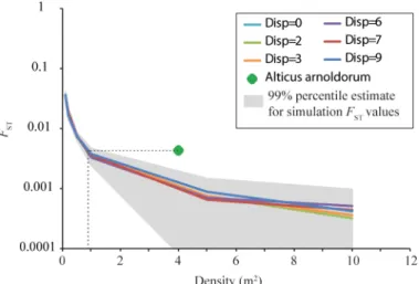
In each of our computer simulations,FSTwas more dependent on grid population density than dispersal scenario (Fig 5): globalFSTdecreased as grid density increased. In other words, as the available habitat became increasingly populated, the increase in effective population size ensured a greater likelihood of gene flow among populations. To obtain a globalFST compara-ble to that computed empirically forA.anolodorum(0.0043), our simulations suggest a popula-tion density just below one individual m-2(Fig 5). The average population density of adultA.
arnoldorumis more likely closer to five individuals m-2[44], which would be consistent with a
simulatedFSTbelow 0.001 (Fig 5). This could reflect a number of things: (i) that the overall dis-persal rate ofA.arnoldorumwas lower than those simulated; (ii) the density of larval fish was Fig 4. Spatial autocorrelation analysis.Based on 204Alticus arnoldorumsamples for microsatellite data excluding putative null alleles. Autocorrelationr
values (black line) are presented in relation to the 95% confidence belt (dotted lines). Error bars at each distance class represent the confidence interval around the observed value ofrbased on 999 bootstrap permutations of the data. The probability values for a one-tailed test for positive autocorrelation, together with upper and lower bounds for the confidence intervals and bootstrap re-sampling are inS5 Table.
lower than settled adult populations; or (iii) that the distribution of individuals was fragmented around the circumference of Guam.
Meta-analysis
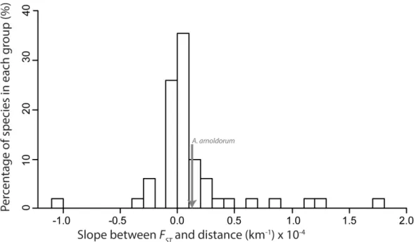
Using the meta-analysis to calculate a generalised trend ofFSTslope over geographic distance (β) not surprisingly we found considerable variation across the published studies: slopes ranged as low as -0.0049 km-1(negative slopes are consistent with recruitment to natal sites) to as high as 0.0017 km-1(suggesting possible active dispersal from natal sites). However, the majority ofβvalues were clustered close to zero with the interquartile range lying between -6.0 x 10⁻⁷km-1and 2.1 x 10⁻⁵km-1 (Fig 6;Table 2). Reef-associated tropical species were also analysed separately to check for any cor-relation between reef lifestyle andβyet their medianβwas 4.04 x 10⁻⁶km-1and still within the interquartile range for all fish species. This was also the case forA.arnoldorumthat was computed to have a slope of 0.12 x 10⁻⁴km-1and found to have no IBD using Mantel tests (see‘Population genetic structure‘above’).
From the 66 studies included in our meta-analysis, 74% were found to have a positiveβas measured usingEq 1while the remaining 26% were found to have a negativeβ(Fig 6;Table 2). Of these 66 studies, 20% reported no spatial genetic structure (no significant pairwiseFST com-parisons), 15% reported little to no spatial genetic structure (few significant pairwiseFST com-parisons), while 65% reported spatial genetic structure (the majority of pairwiseFST
comparisons were significant) (S6 Table). The most common explanations for spatial genetic structure included biogeographic history, habitat boundaries and oceanographic patterns. Only 37 of the 66 studies specifically tested for IBD (using a Mantel test or similar), and of these, just 16 studies reported a significant correlation between geographic distance andFST. Consistent with this, we found that the medianβwas higher in studies that report IBD (median β= 0.19; CI = 0.011–1.14) compared to studies that found no evidence of IBD (medianβ= 0.015; CI = 0.0–0.98;Table 2), although this latter result was marginally non-significant in two-tailed tests (P= 0.08 IBD vs. No IBD,P= 0.11 IBD vs. No IBD and Panmixia). However, the medianβin studies that identified IBD was significantly different from zero (P= 0.003;
Table 2), unlike studies that did not find IBD in whichβwas non-significantly different from Fig 5. Results of simulation analyses ofA.arnoldorumaround Guam illustrating the relationship between density (m3) andF
ST.Each coloured line represents a different dispersal scenario employed in simulations and the green diamond represents the global empiricalFSTforA.arnolodorum. Dispersal distribution‘0’,‘2’,‘3’,‘6’,‘7’, and‘9’correspond to mean squared parent-offspring dispersal distances of 10 m, 40 m, 100 m 200 m, 1000 m respectively.
zero (Table 2). These were important results as they confirmed that our two-point estimate of β(Eq 1) was generally consistent with the overall spatial genetic structure reported in each study.
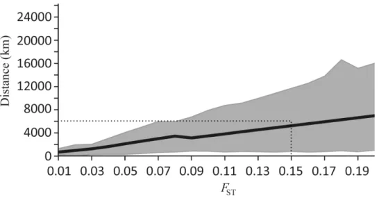
By extrapolating the complete meta-analysis data set and assuming that the relationship betweenFSTand distance is linear in our two point per species data set (or at least locally linear for smallFSTvalues), we predicted the geographic distance at which a givenFSTis likely to be observed (Fig 7;S7 Table). This showed that, in general,FSTaccumulates slowly across vast oceanic distances for fish, although this result should be interpreted with some degree of cau-tion due to the wide confidence intervals associated with ourβmedian estimates. Nonetheless, to obtain a level of genetic isolation generally considered to be important for evolution, i.e. FST= 0.15 [2], the data suggests that the minimum distance between populations for the
“median fish”would need to be at least 5242 km (95% C.I. 810–11692 km;Fig 7). Despite the considerable variance inβamong studies, even the lower confidence interval of this estimate Fig 6. Histogram of meta-analysis data.Showing 90% of the slopes betweenFSTand distance (km). 10% of
data has been excluded for visual clarity (2% below and 8% above histogram range). Excluded outlier values are: -4.9×10⁻³; -3.2×10⁻³; 3.2×10⁻⁴;3.8×10⁻⁴; 6.0×10⁻³;1.3×10⁻³; and 1.7×10⁻³.
doi:10.1371/journal.pone.0150991.g006
Table 2. Rates ofFSTover geographic distance (β) collected in the meta-analysis of marine fish. For the combined data set, the number of studies equals the number of species (slopes averaged across studies; seeMaterials and methods).
Combined Data Studies identifying IBD
Studies identifying no IBD (and Panmixia)
Studies in which IBD was not tested
Number of studies 58 16 25 25
Medianβ(km-1) × 10−4(bootstrap 95% C.I.)
0.016 (0.0044 to 0.096)
0.19 (0.011 to 1.14) 0.015 (0 to 0.098) 0.015 (0 to 0.063) Interquartile rangeβ(km-1) × 10−4 -0.006 to 0.21 0.009 to 1.19 -0.022 to 0.15 -0.0084 to 0.09
Minimumβ(km-1) -0.0049 -2.0 × 10⁻⁶ -1.01 × 10⁻⁴ -0.0061
Maximumβ(km-1) 0.0017 0.0013 2.7 × 10⁻⁴ 0.0017
P-value for medianβdifference from zero
0.004 0.003 0.21 0.28
suggests a degree of connectivity that is much higher than generally appreciated in the litera-ture (e.g., connectivity in marine fishes is likely to be much higher than 300 km; see Introduc-tion). Publication bias could not be measured meaningfully for this data set due to the association between sample size and effect size. Nonetheless, publication bias in this context (i.e. an underrepresentation of published studies that found no spatial genetic structure— trans-lated toFSTslopes of zero in our meta-analysis) would result in our overall estimate ofFST slope with distance presented in the article to be greater than it should be. This would mean thatFSTaccumulates even more slowly across vast oceanic distances already supporting our conclusion (i.e. no publication bias should have no impact on our qualitative result).
Discussion
By comparing empirical data of a species whose ecology effectively eliminates adult dispersal (the land fish,Alticus arnoldorum) to biologically informed simulations and a large meta-anal-ysis of published literature, we provide a broad estimate of the patterns and spatial scale of genetic connectivity at sea. Our comparison was framed around three alternative scenarios of how the behaviour of pelagic larvae might impact genetic connectivity among marine popula-tions. Our results suggest that a scenario involving both passive and active larval dispersal explains the extensive connectivity among populations ofA.arnoldorum(Scenario 3 inFig 2), and possibly many published studies on marine fish more generally (e.g. [13,80–82]). This implies that the high genetic connectivity often assumed to occur in marine environments [9–
12] and confirmed by the results of our meta-analysis, can be maintained by a pelagic larval phase even when adult populations are separated from one another by ecological barriers. Moreover, our meta-analysis provides a broad estimate on the spatial scale necessary for evolu-tionary meaningful genetic differentiation to occur among populations of marine fish. This result has important implications for how we make generalisations about speciation in marine environments. In other words, understanding the rate at which genetic differentiation accumu-lates in the sea provides us with a means to estimate the effect of geographic distance on specia-tion for fish.
Fig 7. Geographic distances (km) expected between populations of marine fish with increasingFST
based on meta-analysis data.The black line represents the median distance expected for anFSTvalue and
is presented in relation to the 95% confidence intervals (grey dotted line) (S7 Table). AnFSTof 0.15 has been marked on the graph as it generally is considered to be significant [2].
Population genetics and demographic history of
Alticus arnoldorum
While our results clearly showed an absence of spatial genetic structuring and IBD in both microsatellite and mitochondrial DNA among sampled sites ofA.arnoldorumaround Guam (Fig 2;S2 Fig;S3andS4Tables), some“chaotic genetic patchiness”was nevertheless detected (Fig 4). The rate of IBD inA.arnoldorumalso fell well within the interquartile range ofβfor published studies for marine fish (Fig 6). Given the ecological isolation of adultA.arnoldorum populations on land, this strongly indicates dispersal among populations via pelagic larvae. However, the absence of strong spatial genetic structure might also reflect one of the following: high effective population sizes, or a lack of sufficient time for genetic drift to have accumulated between isolated populations. Given the demographic expansion or colonization of Guam by
A.arnoldorum(Mismatch analysis, BSP:S1 Fig) we can calculate the expected time (T) for a
pair of populations to reach 50% of the drift-dispersal equilibriumFSTusing the following equation [83]:
T¼ lnð0:5Þ
lnf½ð1 mÞ2 1 1 2Ne
g eq 3
If we assume a maximum larval density forA.arnoldorumof five larvae m-2(e.g. [44]), that dispersal between a pair of populations (m) is 1% per generation and that the effective popula-tion size (Ne) is 10% of the maximum populapopula-tion density [2] thenTis approximately 23 gener-ations. This would be well within the timescale predicted using Bayesian Skyline Plot analysis (S1 Fig). It seems more likely then that the genetic homogeneity observed on Guam is the prod-uct of high larval-based gene flow and high effective population sizes. Both high larval-based gene flow and high effective population sizes appear to independently contribute to genetic homogeneity in many marine taxa [9,24,84].
The patterns of ocean circulation around Guam are generally both spatially and temporally variable with an overall flow that fluctuates from westward to northward at speeds of 0.1–0.2 ms-1[85]. At the lowest flow speed of 0.1 ms-1, it is possible for a passively drifting particle to travel ~242 km during the time of the average pelagic larval phase of anA.arnoldorum(one month; Platt and Ord, unpublished data). This distance is less than the 300 km estimated under a Lagrangian dispersal model for the same time frame [43] yet still further than the max-imum coastal distance between any two of our sample sites (91 km). It therefore seems that Guam represents a single genetic population ofA.arnoldorumdespite adult populations being ecologically isolated from one another. This is common in coral reef fish [5,81,86,87], where significant genetic structuring can often only be detected at the largest of spatial scales [12,88–
92].
Our simulations of genotypic data (Fig 5) were also consistent with scenario 3. The empiri-cal estimate of genetic differentiation among populations ofA.arnoldorumwas always higher than those simulated which again implies chaotic genetic patchiness (Fig 4).
Genetic connectivity in the marine environment
Despite many studies detailing species-specific relationships between genetic connectivity and spatial population structure in the marine environment, there is still limited information about the prevailing patterns with respect to spatial gradients. In general, dispersal estimates based on IBD regressions (Mantel tests or similar) have been shown to reflect direct estimates of dis-persal in mammals (e.g. [97]), reptiles (e.g. [98]), insects (e.g. [99]) and plants (e.g. [100]). Yet, whether or not IBD reflects the typical spatial organisation of marine fish is debateable (e.g. [78]). The results from our meta-analysis provide the first examination of these trends and we estimate the generalised spatial scale at which population genetic structure accumulates over distance for a fish in the ocean. Although our results are a generalisation and do not account for nuanced species specific life history traits, the outcome of our meta-analysis is still an important step towards understanding the scope of connectivity in the marine environment. Arguably, quantifying and understanding the relationship between connectivity and geo-graphic scale is recognised as one of the most critical issues in marine ecology to date [18]. Put simply, spatial information of this sort could be used to determine the scale over which popula-tions of marine fish may interact, the scale over which fisheries should be managed, and the way in which marine protected networks should be designed and implemented [18].
Overall, our meta-analysis agrees with general assumptions about marine dispersal and sug-gests that connectivity is high and genetic differentiation with geographic isolation appears to accumulate slowly at sea for fish in general. For the majority of studies,β(the rate at which genetic differentiation accumulates with distance:Eq 1) clustered closely to zero (Fig 6;
Table 2;S6 Table). This result may be consistent with the assumption that there are few obvi-ous physical barriers in the ocean and that pelagic larval dispersal can lead to high genetic con-nectivity over large geographic distances. Moreover, this appears to occur among adult populations that may be otherwise isolated from one another by ecological barriers. Indeed,β
inA.arnoldorumsits within the interquartile range of published studies (Fig 6), yet it is also a
species where adult populations are ecologically isolated from one another. The implication of this result is that marine fish populations may still be isolated as adults but otherwise connected by larval dispersers that cross or circumvent the ecological barriers separating adult popula-tions. Our finding that larval dispersal inA.arnoldorumis likely a combination of passive and active dispersal (prediction 3; (Fig 3i and 3ii)) is consistent with the well established notion that at least some degree of larval dispersal either active, passive or a combination of both (i.e. >150 km [101]) is also widespread in marine fish (e.g. larval coral reef fishes; [81,101]) and this can translate into genetic connectivity that is vast over large spatial scales for many species.
found that theβwas considerably higher and significantly different to zero in studies that found IBD compared to those that did not (Table 2). This result suggests that populations exhibiting a stepping stone model of dispersal will accumulate genetic structure more rapidly over distance compared to those that do not, even when equal amounts of spatial genetic struc-ture are present.
The variety of causes likely to account for the spatial genetic structure observed in each study (i.e. species specific life history traits) presumably underlies the considerable variance in βin our meta-analysis (Fig 6;Table 2). This was evident in the wide confidence intervals associ-ated with our prediction of the extent to whichFSTwill increase with geographic distance (Fig
7). Indeed, this is a limitation of pooling data across species to obtain a highly generalised pic-ture of dispersal. Nevertheless, we can tentatively estimate the spatial scale at which appreciable genetic differentiation (based on microsatellite markers) might accumulate between popula-tions for a median marine fish (e.g.FST= 0.15; [2]). Our meta-data suggest that populations would need to be approximately 5,000 km apart, with a lower and upper estimate of 810 and 11,692 km, respectively (Fig 7). This result must be interpreted with caution given the assump-tion of linearity applied here and the scale over which most studies are conducted (hundreds of kilometres). Thus, the extrapolation of the relationship to thousands of kilometres may indeed limit the accuracy of our result. Moreover, given the broad confidence intervals of this median estimate, it is important to remember that strong population structure can occur on the scale of tens of kilometres (e.g. [103]), and population structure need not necessarily be present over 5,000 km (e.g. [104]). However, despite applying an assumption of linearity here and the vari-ability on a case by case basis, the overall pattern is consistent with the notion that particularly vast distances are necessary to achieve appreciable genetic structure among populations, and this probably reflects the high dispersal capacity of larvae and the general absence of physical barriers to this mode of dispersal in the marine environment.
It is also important to recognise that lowFSTvalues are generally expected for highly hetero-zygous markers such as microsatellites [28], which can also limit the resolution of weak genetic structure–a characteristic typical of marine organisms [105]. This particular characteristic of our data would bias the meta-analysis to a shallower slope and thus a higher inferred connec-tivity distance for any given pairwiseFSTcomparison. In addition, frequently used measures of genetic connectivity includingFSTmay also over-estimate population connectivity (e.g. demo-graphic processes, also known as“demographic connectivity”). This is because it takes only a few migrants between populations per generation to prevent the accumulation of appreciable genetic differentiation as presumed byFST[106]. Indeed, infrequent stochastic dispersal events may be maintaining genetic exchange across vast distances between otherwise isolated popula-tions [24,106] and as a result, long distance passive larval dispersal may actually be rare and have little demographic input [24,25]. Taken together, estimates of connectivity based on microsatellite data should be interpreted as outer limits for which other measures of connectiv-ity (e.g. the movement of individuals between populations that is of demographic significance) will generally not exceed.
Conclusion
There can be certain caveats associated with making generalisations about connectivity based onFST(e.g. inflation of connectivity estimates [28], non-adherence of data to stepping stone model [24,78,106] and amalgamation of species specific life history traits). However, by employing the combined approach of empirical data, simulations and a meta-analysis we have evaluated the extent to which pelagic larval dispersal in fish likely impacts genetic connectivity among populations that may otherwise be isolated from each other. Using the unusual land fish,A.arnoldorum, as a model, and comparing these results with a meta-analysis, we have been able to assess general patterns of spatial genetic structure in marine fish and provide a broad estimate of the spatial scale of genetic connectivity that would be impossible using a sin-gle approach [107]. This estimate of genetic connectivity is useful for understanding both spe-ciation as well as the conservation implications of spatially oriented resource management in the marine environment. In fact, measures of genetic connectivity such asFSTare being readily incorporated into the design of marine protected areas and reserves e.g. [8,16,18,21,24,108]. With major declines observed in fishery stocks, the accelerated degradation of coastal habitat and climate change, understanding the complexity of connectivity in marine organisms, including genetic connectivity, has never been more critical for the conservation and manage-ment of marine environmanage-ments. Indeed, understanding genetic connectivity in this context will ultimately assist us to diagnose the resilience of populations and species in our marine habitats.
Supporting Information
S1 Fig. PRISMA 2009 Checklist. (DOC)S2 Fig. Bayesian skyline plot derived from the ATPase 6 and 8 sequences (n= 120) showing the effective population size as a function of time.The thick black line is the median estimate of the log10of the effective population size, and the thin grey lines are the 95% higher posterior density.
(TIF)
S3 Fig. STRUCTURE results based on 204Alticus arnoldorumsamples for microsatellite data excluding putatively null alleles: (i) K = 2 after Evanno et al. [68] and (ii) K = 6. Individu-als are grouped by sampling location and each individual is represented by one vertical line bro-ken into K coloured segments, with the lengths being proportional to the K inferred cluster. (TIF)
S1 Table. Characterisation of the 17 polymorphic microsatellite loci forAlticus arnoldorum (N = 204) and multiplex panel design.Types of fluorescence used to label forward primers are indicated with the primer sequence (FAM, NED, PET, VIC). NA, number of alleles. (DOCX)
S2 Table. Descriptive statistics and diversity indices for each population per locus.Na, num-ber of alleles per locus; Ar, allelic richness;FIS,Wrights inbreeding coefficient; HW Obs, Hardy-Weinberg observed heterozygosity; HW Exp. Hardy-Weinberg expected heterozygos-ity; and HW p-value, Hardy-Weinberg P-value;, significant after sequential Bonferonni
cor-rection. (DOCX)
S3 Table. PairwiseFSTcomparisons for the 7 sampled populations ofAlticus arnoldorum. No comparisons were significantly different.
S4 Table. Pairwise FSTcomparisons for the 7 sampled populations ofAlticus arnoldorum,
(i) total data set, (ii) data set excluding null alleles (P0.05 after bonferroni correction). (DOCX)
S5 Table. Spatial Autocorrelation analysis for the microsatellite data set excluding putative null alleles.The number of pairwise comparisons,N, correlation, r, upper U and lower L bounds for a 95% confidence interval (H0: r = 0), the upper Ur and lower Lr bounds deter-mined by bootstrap resampling, the probability P of a one-tailed test for positive autocorrela-tion, and the x-intercept are shown across all distance classes.
(DOCX)
S6 Table. Meta-analysis data including each study used, the FST slope calculated asβ ¼
ΔFST
ΔDistanceand the spatial pattern identified in each study. (DOCX)
S7 Table. Distance predictions according toFSTbased on meta-analysis data. (DOCX)
Acknowledgments
We would like to thank C. Riginos and J. M. Leis for their comments on the manuscript, J. McIlwain for logistical support in Guam and M. Taylor for help in catching specimens. This work was supported by Evolution and Ecology Research Centre start-up funds, a University of New South Wales Science Faculty Research Grant and Australian Research Council major grant to TJO. This study was covered by the UNSW Animal Care and Ethics Committee proto-col 11/36B.
Author Contributions
Conceived and designed the experiments: GMC TJO. Performed the experiments: GMC. Ana-lyzed the data: GMC TES. Contributed reagents/materials/analysis tools: TJO WBS. Wrote the paper: GMC TES TJO WBS.
References
1. Avise JC. Phylogeography: The History and Formation of Species. Harvard University Press; 2000. 2. Frankham R, Ballou JD & Briscoe DA. Introduction to Conservation Genetics, 2ndEd. Cambridge
University Press; 2010.
3. Jones GP, Almany GR, Russ GR, Sale PF, Steneck RS, van Oppen MJH et al. Larval retention and connectivity among populations of corals and reef fishes: history, advances and challenges. Coral Reefs. 2009; 28: 307–325.
4. Harrison HB, Williamson DH, Evans RD, Almany GR, Thorrold SR, Russ GR, et al. Larval Export from Marine Reserves and the Recruitment Benefit for Fish and Fisheries. Curr Biol. 2012; 22: 1023–1028. doi:10.1016/j.cub.2012.04.008PMID:22633811
5. Leis J.M. & McCormick M.I. 2002. The biology, behavior, and ecology of the pelagic larval stage of coral reef fishes. In: Sale PF editor. Coral Reef Fishes: Dynamics and Diversity in a Complex Ecosys-tem. Academic Press; 2002. pp. 171–199
6. Cowen RK, Paris CB & Srinivasan A. Scaling of connectivity in marine populations. Science. 2006; 311: 522–527. PMID:16357224
7. Cowen RK, Gawarkiewic G, Pineda J, Thorrold SR & Werner FE. Population Connectivity in Marine Systems An Overview. Oceanography. 2007; 20: 14–21.
8. Fogarty MJ & Botsford LW. Population Connectivity and Spatial Management of Marine Fisheries. Oceanography. 2007; 20: 112–123.
10. Waples RS. Separating the wheat from the chaff: Patterns of genetic differentiation in high gene flow species. J Hered. 1998; 89: 438–450.
11. Hellberg ME. Footprints on water: the genetic wake of dispersal among reefs. Coral Reefs. 2007; 26: 463–473.
12. Puebla O, Bermingham E & Guichard F. Estimating dispersal from genetic isolation by distance in a coral reef fish (Hypoplectrus puella). Ecology. 2009; 90: 3087–3098. PMID:19967864
13. Leis JM. Are larvae of demersal fishes plankton or nekton? Adv Mar Biol. 2006; 51: 57–141. PMID:
16905426
14. Jones GP, Milicich MJ, Emslie MJ & Lunow C. Self-recruitment in a coral reef fish population. Nature. 1999; 402: 802–804.
15. Swearer SE, Caselle JE, Lea DW & Warner RR. Larval retention and recruitment in an island popula-tion of a coral-reef fish. Nature. 1999; 402: 799–802.
16. Cowen RK & Sponaugle S. Larval Dispersal and Marine Population Connectivity. Ann Rev Mar Sci. 2009; 1: 443–466. PMID:21141044
17. Wright S. Evolution in Mendelian populations. Genetics. 1931; 16: 97–159. PMID:17246615
18. Leis JM, Van Herwerden L & Patterson HM. Estimating connectivity in marine fish populations: What works best? In: Gibson RN, Atkinson RJA & Gordon JDM editors. Oceanography and Marine Biology: An Annual Review. Vol 49, 2011; pp. 193–234.
19. Bohonak AJ. Dispersal, gene flow, and population structure. Q. Rev. Biol. 1999; 74: 21–45. PMID:
10081813
20. Weersing K & Toonen RJ. Population genetics, larval dispersal, and connectivity in marine systems. Mar Ecol Prog Ser. 2009; 393: 1–12.
21. Selkoe KA & Toonen RJ. Marine connectivity: a new look at pelagic larval duration and genetic met-rics of dispersal. Mar Ecol Prog Ser. 2011; 436: 291–305.
22. Wright S. Isolation by Distance. Genetics. 1943; 28: 114–38. PMID:17247074
23. Rousset F. Genetic differentiation and estimation of gene flow from F-statistics under isolation by dis-tance. Genetics. 1997; 145: 1219–1228. PMID:9093870
24. Palumbi SR. Population genetics, demographic connectivity, and the design of marine reserves. Ecol App. 2003; 13: S146–S158.
25. Puebla O, Bermingham E & McMillan WO. On the spatial scale of dispersal in coral reef fishes. Mol Ecol. 2012; 21: 5675–5688. doi:10.1111/j.1365-294X.2012.05734.xPMID:22994267
26. Whitlock MC & McCauley DE. Indirect measures of gene flow and migration: F-ST not equal 1/(4Nm+1). Heredity. 1999; 82: 117–125. PMID:10098262
27. Sherwin WB, Jabot F, Rush R & Rossetto M. Measurement of biological information with applications from genes to landscapes. Mol Ecol. 2006; 15: 2857–2869. PMID:16911206
28. Hedrick PW. A standardized genetic differentiation measure. Evolution. 2005; 59: 1633–1638. PMID:
16329237
29. Jost L. G(ST) and its relatives do not measure differentiation. Mol Ecol. 2008; 17: 4015–4026. PMID:
19238703
30. Sherwin WB. Entropy and Information Approaches to Genetic Diversity and its Expression: Genomic Geography. Entropy. 2010; 12: 1765–1798.
31. Whitlock MC. G '(ST) and D do not replace F-ST. Molecular Ecology. 2011; 20: 1083–1091. doi:10. 1111/j.1365-294X.2010.04996.xPMID:21375616
32. Ord TJ & Hsieh ST. A Highly Social, Land-Dwelling Fish Defends Territories in a Constantly Fluctuat-ing Environment. Ethology. 2011; 117: 918–927.
33. Martin K & Lighton J. Aerial CO2 and O2 exchange during terrestrial activity in an amphibious fish,
Alticus kirki(Blenniidae). Copeia. 1989;723–727.
34. Brown CR, Gordon MS & Martin KLM. Aerial and aquatic oxygen uptake in the amphibious Red Sea rockskipper fish, Alticus kirki (Family Blenniidae). Copeia. 1992; 4: 1007–1013.
35. Martin KLM. Time and tide wait for no fish: intertidal fishes out of water. Env Biol Fish. 1995; 44: 165– 181.
36. Hsieh STT. A Locomotor Innovation Enables Water-Land Transition in a Marine Fish. Plos One. 2010; 5:e11197 doi:10.1371/journal.pone.0011197PMID:20585564
38. Lourie SA, Doherty PJ & Bernardi G. Strong genetic divergence among populations of a marine fish with limited dispersal,Acanthrochromis polyacanthus, within the Great Barrier Reef and the Coral Sea. Evolution. 2001; 55:2263–73 PMID:11794786
39. Timm J, Figiel M & Kochzius M. Contrasting patterns in species boundaries and evolution of anemo-nefishes (Amphiprioninae, Pomacentridae) in the centre of marine biodiversity. Mol Phy Evol. 2008; 49:268–76
40. Timm J & Kochzius M. Geological history and oceanography of the Indo-Malay Archipelago shape the genetic populaiton structure in the false clown anemonefish (Amphiprion ocellaris). Mol Ecol. 2008; 17:3999–4014 PMID:19238702
41. Ward RD, Skibinski DOF & Woodwark M. Protein heterozygosity, protein structure, and taxonomic dif-ferentiation. Evol Biol. 1992; 26: 73–159.
42. Peakall R, Ruibal M & Lindenmayer DB. Spatial autocorrelation analysis offers new insights into gene flow in the Australian bush rat,Rattus fuscipes. Evolution. 2003; 57: 1182–1195. PMID:12836834
43. Siegel DA, Kinlan BP, Gaylord B & Gaines SD. Lagrangian descriptions of marine larval dispersion. Mar Ecol Prog Ser. 2003; 260: 83–96.
44. Morgans CL, Cooke GM & Ord TJ. How populations differentiate despite gene flow: sexual and natu-ral selection drive phenotypic divergence within a land fish, the Pacific leaping blenny. BMC Evol Biol. 2014; 14:97 doi:10.1186/1471-2148-14-97PMID:24884492
45. Johnson MS & Black R. Chaotic genetic patchiness in an inter-tidal limpet,Siphonariasp. Mar Biol. 1982; 70: 157–164.
46. Johnson MS & Black R. Pattern beneath the chaos—the effect of recruitment on genetic patchiness in an intertidal limpet. Evolution. 1984; 38: 1371–1383.
47. Bermingham E, McCafferty SS & Martin AP. Fish biogeography and molecular clocks: Perspectives from the Panamanian isthmus. In: Kocher TD & Stepien CA editors. Molecular Systematics of Fishes. Academic Press; 1997
48. Cooke GM, Chao NL & Beheregaray LB. Five Cryptic Species in the Amazonian Catfish Centromo-chlus existimatusidentified based on biogeographic predictions and genetic data. Plos One. 2012; 7: e48800. doi:10.1371/journal.pone.0048800PMID:23144977
49. Gardner MG, Fitch AJ, Bertozzi T & Lowe AJ. Rise of the machines–recommendations for ecologists when using next generation sequencing for microsatellite development. Mol Ecol Res. 2008; 11: 1093–1101.
50. Templeton AR, Crandall KA & Sing CF. A cladistic analysis of phenotypic associations with haplo-types inferred from restriction endonuclease mapping and DNA sequence data. III. Cladogram esti-mation. Genetics. 1992; 132: 619–33. PMID:1385266
51. Clement M, Posada D & Crandall KA. TCS: a computer program to estimate gene genealogies. Mol Ecol. 2000; 9: 1657–9. PMID:11050560
52. Nei M. Molecular Evolutionary Genetics. Columbia University Press; 1987.
53. Excoffier L, Laval LG & Schneider S. Arlequin ver. 3.0: An integrated software package for population genetics data analysis. Evol Bioinf Online. 2005; 1: 47–50.
54. Rodgers AR & Harpending H. Population growth makes waves in the distribution of pairwise genetic differences. Mol Biol Evol. 1992; 9, 552–569. PMID:1316531
55. Fu Y-X. Statistical tests of neutrality of mutations against population growth, hitchhiking and back-groud selection. Genetics. 1997; 147, 915–925. PMID:9335623
56. Drummond AJ, Rambaut A, Shapiro B & Pybus OG. Bayesian coalescent inference of past population dynamics from molecular sequences. Mol Biol Evol. 2005; 22, 1185–1192. PMID:15703244
57. Drummond A & Rambaut A. BEAST: Bayesian evolutionary analysis by sampling trees. BMC Evol Biol. 2007; 7, 214–221. PMID:17996036
58. Rambaut A, Suchard MA, Xie D & Drummond AJ. Tracer v1.6. 2014. Available:http://beast.bio.ed.ac. uk/Tracer
59. Excoffier L, Smouse PE & Quattro JM. Analysis of molecular variance inferred from metric distances among DNA haplotypes: application to human mitochondrial DNA restriction data. Genetics. 1992; 131: 479–491. PMID:1644282
60. Raymond M & Rousset F. GENEPOP (version 1.2): population genetics software for exact tests and ecumenicism. J Hered. 1995; 86: 248–249.
61. Rousset F. Genepop'007: a complete reimplementation of the Genepop software for Windows and Linux. Mol Ecol Res. 2008; 8: 103–106.