PROGRAMA DE PÓS-GRADUAÇÃO EM ECOLOGIA
ELIANA FARIA DE OLIVEIRA
FILOGEOGRAFIA DE CNEMIDOPHORUS OCELLIFER
(SQUAMATA: TEIIDAE) NA CAATINGA
ELIANA FARIA DE OLIVEIRA
FILOGEOGRAFIA DE CNEMIDOPHORUS OCELLIFER
(SQUAMATA: TEIIDAE) NA CAATINGA
Tese apresentada ao programa de Pós-Graduação em Ecologia da Universidade Federal do Rio Grande do Norte, como parte das exigências para a obtenção do título de Doutor em Ecologia.
Orientador: Dr. Gabriel Correa Costa
Co-orientadores: Dr. Daniel O. Mesquita Dr. Frank T. Burbrink
Catalogação da Publicação na Fonte. UFRN / Biblioteca Setorial do Centro de Biociências
Oliveira, Eliana Faria de.
Filogeografia de Cnemidophorus ocellifer (Squamata: Teiidae) na Caatinga / Eliana Faria de Oliveira. – Natal, RN, 2014.
169 f.: il.
Orientador: Dr. Gabriel Correa Costa. Coorientador: Dr. Daniel O. Mesquita. Coorientador: Dr. Frank T. Burbrink.
Tese (Doutorado) – Universidade Federal do Rio Grande do Norte. Centro de Biociências. Programa de Pós-Graduação em Ecologia.
1. Estrutura genética. – Tese. 2. Fluxo gênico. – Tese. 3. Répteis. – Tese. I. Costa, Gabriel. II. Mesquita, Daniel O. III. Burbrink, Frank T. IV. Universidade Federal do Rio Grande do Norte. V. Título.
ELIANA FARIA DE OLIVEIRA
FILOGEOGRAFIA DE CNEMIDOPHORUS OCELLIFER
(SQUAMATA: TEIIDAE) NA CAATINGA
Tese apresentada ao programa de Pós-Graduação em Ecologia da Universidade Federal do Rio Grande do Norte, como parte das exigências para a obtenção do título de Doutor em Ecologia.
Data da defesa: 31 de outubro de 2014. Resultado: ____________________
______________________
______________________
Dr. Felipe Gobbi Grazziotin Dr. Guarino Rinaldi Colli
______________________________ _____________________________ Dr. Adrian Antonio Garda Dr. Sérgio Maia Queiroz Lima
_______________________
i
“Fazer da interrupção um caminho novo. Fazer da queda um passo de dança, do medo uma escada, do sono uma ponte, da procura um encontro.”
ii
AGRADECIMENTOS
Foram alguns momentos de lucidez e muitos outros nem tão inspirados... Mas em todos eles pude
sempre contar com uma palavra de incentivo ou um ombro amigo. Por isso, gostaria de expressar
a minha imensa gratidão a todos aqueles que foram fundamentais para que esse trabalho se
realizasse.
Ao Gabriel Costa, por ter aceitado e encarado esse desafio ao meu lado, estando sempre presente.
Obrigada pelos ensinamentos, direcionamentos e pelo apoio nos momentos de insegurança.
Ao Marcelo Gehara e Pablo Martinez pela inestimável ajuda com as análises e discussões. Muito
obrigada pela amizade e por compartilharem comigo seus conhecimentos sobre filogeografia e
estatística.
Ao Frank Burbrink, Daniel Mesquita, Adrian Garda e Sérgio Lima, pelas sugestões e
contribuições em diferentes etapas deste trabalho.
Ao Vinícius São Pedro, pelo seu sincero amor, carinho e amizade. Você sabe que metade dessa
tese também é sua e que você também é metade de mim.
Aos meus pais, Valdir e Odila, por serem meu maior exemplo de persistência e sabedoria. Às
minhas irmãs, Elisa e Larissa, pelas inúmeras palavras de incentivo e carinho. Vocês são o meu
alicerce e minha força maior para seguir adiante!
Aos amigos do LAR-UFRN e do Costa Lab: Diego Santana, Sarah Mângia, Felipe Magalhães,
iii
Pedro Medeiros, Alan Filipe, Anne Karenine, Marcos de Brito, Felipe Figueiredo, Willianilson
Pessoa, Jéssica Coelho, Juan Pablo Zurano, Adrián García-Rodríguez, Carolina Lisboa, Brunno
Freire e Caterina Penone. Obrigada pela agradável convivência e amizade!
Aos amigos do doutorado-sanduíche, Pedro Peloso, Sílvia Pavan, Anelise Hahn, André Carvalho,
pela ajuda e acolhida. Pessoal do laboratório, Edward Myers, Alex McKelvy, Xin Chen, Ivana
Novcic, Ashley Ozelski, Guo Peng, Sara Ruane, pela paciência e companheirismo. Maria
Chernova, nossa anfitriã, pelo imenso carinho.
Aos amigos Phoeve Macário, Guilherme Toledo, Andreia Estrela, Priscilla Vilela, Daniel Freire,
Guilherme Mazzochini, Adriana Pellegrini, Gustavo Paterno, Lígia Rocha, Rafael Laia, Miriam
Plaza, Daniel Lanza e tantos outros amigos, colegas e parentes, pela torcida, pela preocupação e
todo tipo de ajuda.
Aos professores e alunos da Pós-Graduação em Ecologia, pela amizade, ensinamentos,
discussões e incentivo.
Aos curadores, estagiários e funcionários das instituições que gentilmente enviaram amostras de
tecidos: Universidade de Brasília (UnB), Universidade de São Paulo (USP), Universidade
Católica do Salvador (UCSAL), Universidade Federal da Paraíba (UFPB), Universidade Federal
do Rio Grande do Norte (UFRN), Universidade Federal de Alagoas (UFAL), Universidade
Federal de Viçosa (UFV), Universidade Federal de Sergipe (UFS), and Universidade Federal do
iv
À Coordenação de Aperfeiçoamento de Pessoal de Nível Superior (Capes), pela bolsa de
doutorado concedida e ao Conselho Nacional de Desenvolvimento Científico e Tecnológico
(CNPq), pelos recursos financiadores deste projeto.
Todos vocês contribuiram com esta conquista, tornando esta trajetória menos árdua. Muito
v SUMÁRIO
LISTA DE TABELAS...viii
LISTA DE FIGURAS...xiii
SÍNTESE...xvii
CAPÍTULO I: Speciation with gene flow in whiptail lizards from a Neotropical xeric biome...1
Abstract...3
Introduction...4
Materials and Methods...7
Sample collection and sequencing...7
Population structure and assignment...8
Genetic diversity and genetic distances...9
Gene tree estimation and haplotype genealogy...9
Species tree estimation…...10
Historical demography...11
Migration...12
Phylogeographic reconstructions...12
Tests of diversification scenarios...13
Results...15
DNA polymorphism, population structure and species tree estimation...15
Historical demography and migration...16
Phylogeographic reconstructions...17
Tests of diversification scenarios...18
vi
Environmental changes and diversification...18
Phylogeographic implications...22
Taxonomic implications...24
Species synonymy and distribution...27
Conclusion...27
Acknowledgements...28
Author contributions...29
References...29
Tables and Figures...35
Supporting information...45
Taxonomic Background...45
Fossil Record...47
Tables and Figures...49
CAPÍTULO II: Influence of landscape features on genetic diversity and differentiation in Brazilian whiptail lizard (Cnemidophorus ocellifer)...79
Abstract...81
Introduction...82
Materials and Methods...85
Sample collection and sequencing...85
Genetic diversity and differentiation...85
Ecological niche modelling...86
Effect of historic and environmental factors on genetic diversity...88
vii
Niche stability hypothesis...89
Water and energy availability hypothesis...90
Environmental heterogenety hypothesis...90
Colonization hypothesis...90
Statistical analyses: genetic diversity...91
Effect of isolation by distance versus isolation by resistance on genetic differentiation...92
Isolation by distance hypothesis...93
Isolation by resistance hypotheses...93
Statistical analyses: genetic differentiation....94
Results...94
Genetic diversity and differentiation...94
Ecological niche modelling...95
Effect of historic and environmental factors on genetic diversity...96
Effect of isolation by distance versus isolation by resistance on genetic differentiation...96
Discussion...97
Effect of historic and ecological factors on genetic diversity...97
Isolation by distance versus isolation by resistance...101
Conclusion...102
Acknowledgements...103
Author contributions...104
References...104
Tables and Figures...109
Supporting information...118
viii
LISTA DE TABELAS
CAPÍTULO I:
Table 1. Genetic statistics for each locus for Northeast and Southwest lineages of Cnemidophorus
ocellifer.
Table 2. Variance percentages for components of analyses of molecular variance (AMOVA) performed with different genes in Northeast and Southwest lineages of Cnemidophorus ocellifer.
Table 3. Genetic distance (uncorrected p-distance) between and within Northeast and Southwest lineages of Cnemidophorus ocellifer performed with different genes.
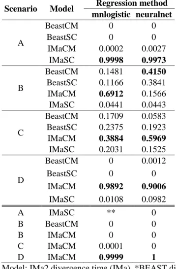
Table 4. Results from ABC analyses assuming four scenarios of diversification (A, B, C, or D;
see Fig. 6) between Northeast and Southwest lineages of Cnemidophorus ocellifer. Values represent posterior probabilities of comparisons within each scenario (tolerance of 0.0001) and among the best models selected for each scenario (tolerance of 0.001). Preferred model at each
comparison is highlighted in bold.
Table S1. Samples of Cnemidophorus used in present study (398 samples + 1 outgroup). For each
sample is presented map code number (see Fig. 1), collection locality, state, institution of origin, voucher number, laboratory code number, and geographic coordinates (longitude and latitude in
ix
Table S2. Primers used for amplification and sequencing of the five loci used in this study. Each
primer presents the source of origin and the annealing temperature (T) in degrees Celsius (°C).
Table S3. Analyses performed in BEAST program. For each analysis is presented the locus used, number of sequences (N), substitution model estimated by jModelTest program, and settings for molecular clock, mutation rate, tree prior, chain size (MCMC) and sampling frequency (Freq).
Table S4. Species used in estimating the 12S substitution rate for Teiidae.
Table S5. Parameters and prior distributions used to test alternative scenarios for diversification of the Northeast and Southwest lineages under ABC approach.
Table S6. Samples of Cnemidophorus used in this study (subset of 137 samples). For each
sample is presented map code number (see Fig. 1), collection locality, state, laboratory code number, populations found by the GENELAND and STRUCTURE analysis, and mtDNA and nuDNA haplotypes (see Fig. 3). Number 2 between parentheses indicates homozygous
individuals.
Table S7. Tests of nested models in IMa2 for Northeast and Southwest lineages.
x CAPÍTULO II:
Table 1. Genetic statistics for the sampling localities of Cnemidophorus ocellifer. Number of
sampled individuals (N), nucleotide diversity (π), haplotype diversity (Hd), and number of
haplotypes (H). Localities and haplotypes network can be visualized in Fig. 1.
Table 2. General hypotheses tested to explain genetic diversity and structure in Cnemidophorus
ocellifer.
Table 3. Percent contribution and permutation importance of each climatic variable used in ecological niche modelling for Cnemidophorus ocellifer.
Table 4. Results of the linear regression or simultaneous autoregression analyses performed to test the genetic diversity in Cnemidophorus ocellifer. The best models are highlighted in bold.
Table 5. Results of the multiple regressions on distance matrices (MRM) performed to test the genetic differentiation in Cnemidophorus ocellifer. The best models are highlighted in bold.
Table S1. Samples of Cnemidophorus ocellifer used in present study (336 samples). A map code number (see Fig. 1) is presented for each sample, along with locality, state, institution of origin,
xi
Table S2. Matrix of pairwise FST distances (bellow the diagonal) and significant FST p-values
(above the diagonal) for the 46 sampled localities of Cnemidophorus ocellifer. Available at http://costagc.weebly.com/publications.html.
Table S3. Occurrence dataset of Cnemidophorus ocellifer used in Ecological Niche Modelling. For each locality the data source and geographic coordinates (in decimal degrees) are presented.
Table S4. Climate and environmental values for each locality used to test genetic diversity in
Cnemidophorus ocellifer through linear regression or simultaneous autoregression analyses. Nucleotide diversity (π); niche suitability from current and Last Glacial Maximum (LGM, 21
kyr) periods; isothermality (Bio3), temperature seasonality (Bio4), minimum temperature of
coldest month (Bio6), annual mean temperature (Bio1), annual precipitation (Bio12), net primary productivity (NPP), actual evapotranspiration (AET), topographic complexity (TC), and distance
from center of origin (DCO). Letters after Bio3, Bio4 and Bio6 variables represent current (C) and LGM (L) climate conditions. Available at http://costagc.weebly.com/publications.html.
Table S5. Linear regression results that confirm the positive and significant association between Ecological Niche Modelling of Cnemidophorus ocellifer and the three most important current (C) climate variables to the model: isothermality (Bio3), temperature seasonality (Bio4), and
minimum temperature of coldest month (Bio6).
Table S6. Matrix of pairwise Euclidian distances for the 46 sampled localities of Cnemidophorus
xii
Table S7. Matrix of pairwise connectivity distance for the 46 sampled localities of
Cnemidophorus ocellifer based on its current niche suitability. Available at
http://costagc.weebly.com/publications.html.
Table S8. Matrix of pairwise connectivity distance for the 46 sampled localities of
Cnemidophorus ocellifer based on its LGM niche suitability. Available at
http://costagc.weebly.com/publications.html.
Table S9. Matrix of pairwise connectivity distance for the 46 sampled localities of
Cnemidophorus ocellifer based on Caatinga main rivers. Available at
http://costagc.weebly.com/publications.html.
Table S10. Matrix of pairwise resistance distance for the 46 sampled localities of Cnemidophorus
ocellifer based on Caatinga slope gradient. Available at
http://costagc.weebly.com/publications.html.
Table S11. Matrix of pairwise resistance distance for the 46 sampled localities of Cnemidophorus
ocellifer based on Caatinga roughness gradient. Available at
http://costagc.weebly.com/publications.html.
Table S12. Standardized coefficients of linear regressions that confirm the positive association
xiii
LISTA DE FIGURAS
CAPÍTULO I:
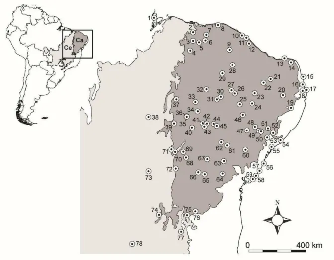
Fig. 1. Distribution of sampled localities for Cnemidophorus ocellifer species complex. Numbers correspond to 78 localities names in Tables S1 and S6, Supporting information. Gray shades represent biomes limits: Caatinga (Ca) in dark gray and Cerrado (Ce) in light gray.
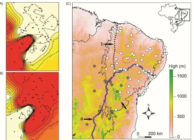
Fig. 2. GENELAND analysis (A and B) with posterior probability isoclines, which indicate
extensions of the genetic populations found (black lines with inclusion probabilities). Light color zones in each map indicate the groups of localities with greater probabilities of belonging to the same genetic unit. Black dots indicate locations of the 78 analyzed localities. Map on the right
(C) shows the distribution of Northeast (white circles) and Southwest (gray circles) lineages along Caatinga (Ca) and Cerrado (Ce) biomes, depicting São Francisco River (a), its hypothetical
paleo-course (b), and Espinhaço Mountain Range (c). Red dotted circle represents the probable geographic origin of Northeast lineage (see also Fig. 5). Green color represents higher altitudes and white represents lower altitudes.
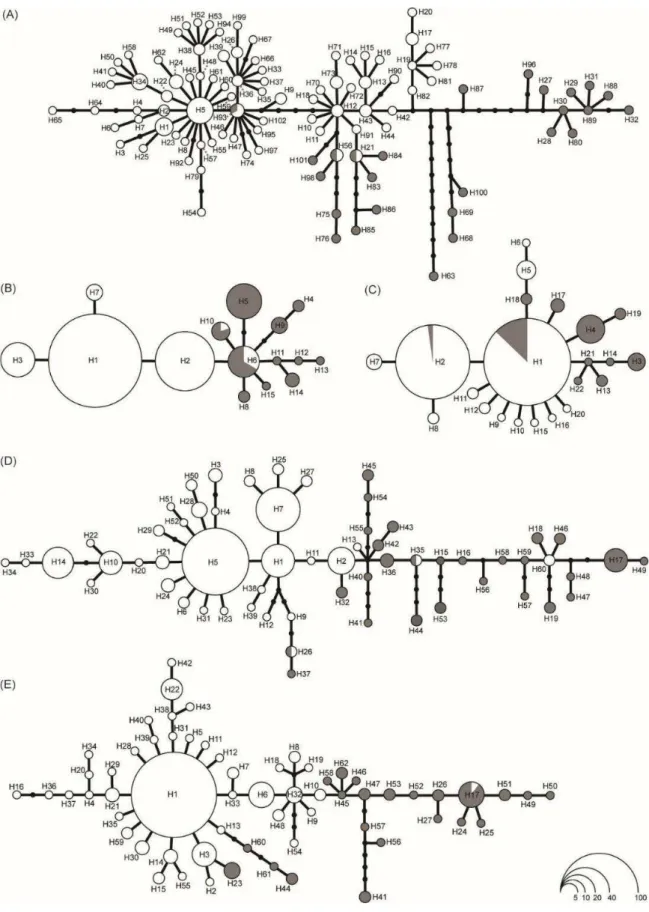
Fig. 3. Haplotype genealogies from maximum likelihood analysis of 12S (A), RP40 (B), R35 (C), ATPSB (D), and NKTR (E) gene trees performed in the software Haploviewer. Each haplotype is
represented by a circle whose area is proportional to its frequency (indicated in legend). White and gray circles represent Northeast and Southwest lineages, respectively. Black dots represent
xiv
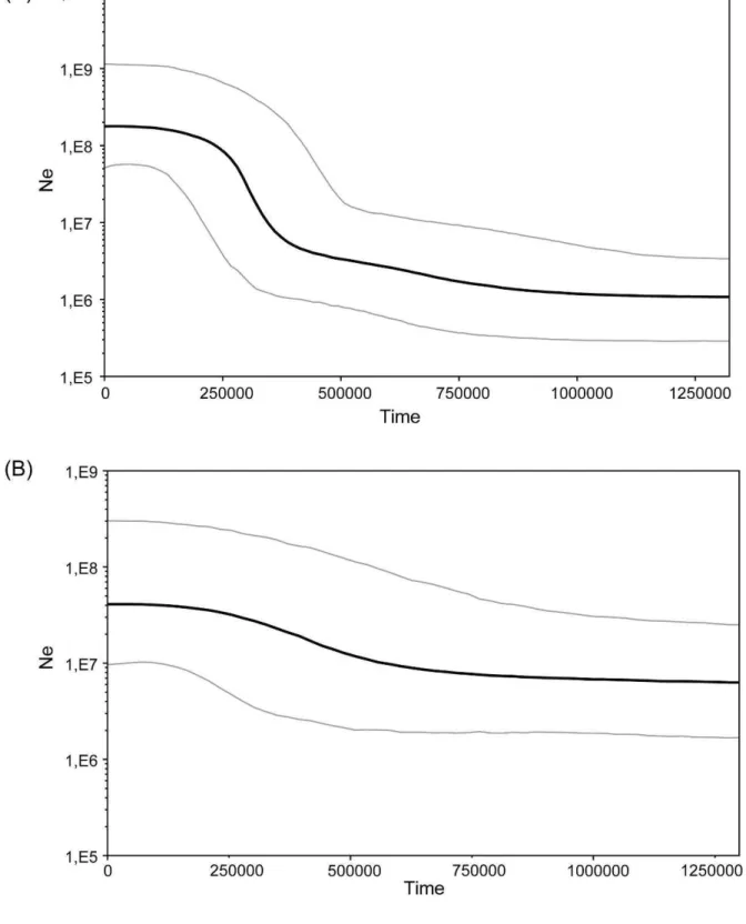
Fig. 4. Bayesian Skyline plots illustrating effective population sizes (Ne) through time (in years)
of Southwest (A) and Northeast (B) lineages. The back line represents the median population size, and the gray lines represent 95% higher posterior probability.
Fig. 5. Phylogeographic reconstructions of Northeast lineage. The spatiotemporal dynamics for the genes 12S (A), ATPSB (B), NKTR (C), R35 (D), and RP40 (E) are shown in four different
time frames since their origin to present. Light polygons represent basal clades and darker ones represent recent clades. Lines represent the maximum clade credibility tree branches projected on
the surface. Maps are based on satellite pictures visualized with Google Earth.
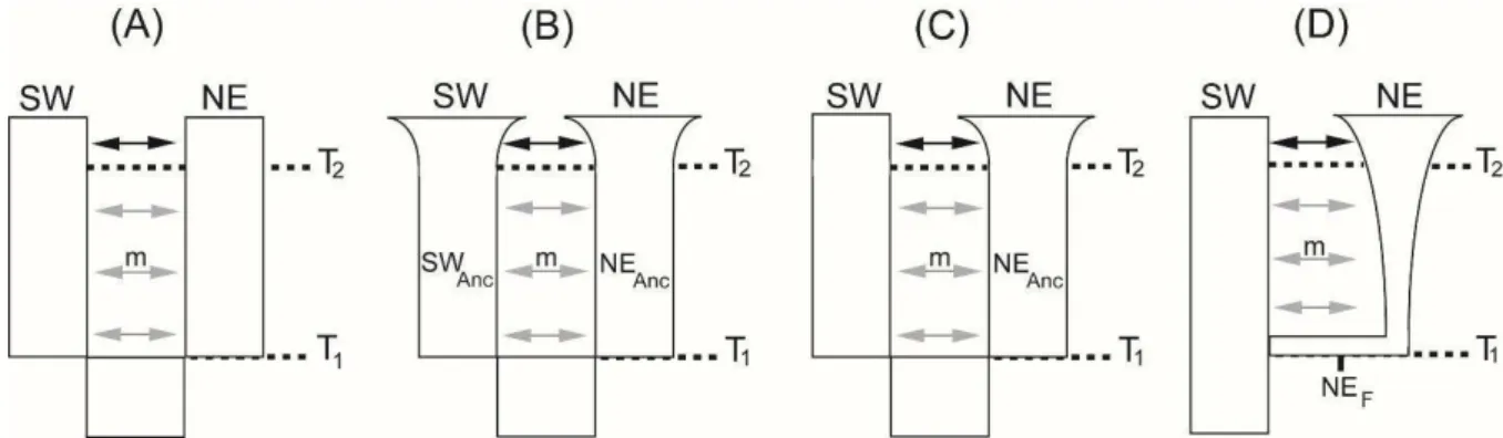
Fig. 6. Alternative scenarios for diversification of the Northeast (NE) and Southwest (SW)
lineages tested with multilocus ABC. Divergence time is referred to as T1, and SWANC and NEANC represent Southwest and Northeast ancestral populations, respectively. Northeast founder
population is referred to as NEF. Models include two migration rates (m) possibilities: migration throughout the population history (gray and black arrows, and migration starts in T1) and recent migration (black arrows, and migration starts in T2). T2 also represents the beginning of the
population expansion (scenarios B and C). Prior distributions for each parameter are available at Table S5, Supporting information. See Materials and Methods for more details.
Fig. S1. Haplotype network for 12S (A), RP40 (B), NKTR (C), R35 (D) and ATPSB (E) using median-joining method. Each haplotype is represented by a circle whose area is proportional to
xv
Fig. S2. STRUCTURE results showing (A) plot of the log-likelihood value (LnPr(X|K)) versus the number of potential populations (K), (B) plot of Evanno ΔK method to evaluate the most
supported K based on rate of change of the likelihood distribution as a function of K, and (C) plot of ancestry estimates, which represent the estimated membership for K-inferred clusters.
Fig. S3. Gene trees for 12S (A), RP40 (B), ATPSB (C), R35 (D) and NKTR (E) inferred using Bayesian inference in the program BEAST. Gray branches represent the Southwest lineage and
the other branches indicate the Northeast lineage. Posterior probabilities of 100% and ≥ 95% are indicated by asterisk and filled circles, respectively. Terminal names of samples (137 in total) are available in Table S6 (Supporting information), together with additional information.
Fig. S4. Principal Components Analysis vectors predictive plots, PC1 × PC2 (A) and PC1 × PC3
(B), for the prior predictive distributions of summary statistics for the five best models (see Table 4) compared using the Approximate Bayesian Computation approach.
CAPÍTULO II:
Fig. 1. Map with localities sampled for genetic data of the whiptail lizard Cnemidophorus
ocellifer along the Caatinga biome (light gray). Haplotypes genealogy from Maximum
Likelihood analysis of the 12S gene tree performed in the software Haploviewer. Each haplotype is represented by a circle whose size is proportional to its frequency (indicated in legend). The
xvi
Fig. 2. Spatial distribution of the genetic variation in Cnemidophorus ocellifer represented by
interpolated π values (A) and interpolated pairwise genetic distance (B).
Fig. 3. Geographic distribution of climatically suitable habitats for Cnemidophorus ocellifer during four temporal scenarios: current, mid-Holocene (6 kyr), Last Glacial Maximum (LGM, 21 kyr) and Last Interglacial (LIG, ~130 kyr). Black dots represent all 91 localities (available at
Table S3, Supporting information) used as species occurrence dataset in niche modelling procedures.
Fig. S1. Correlograms of Moran’s I coefficients calculated for 10 geographic distance classes
(km) through simultaneous autoregression (SAR) between genetic diversity and (A) current niche
suitability, (B) LGM niche suitability (C) refugia, (D) annual precipitation – Bio12, (E) topographic complexity, and (F) distance from center of origin. Spatial autocorrelation was
absent at any distance in all models.
Fig. S2. Correlograms of Moran’s I coefficients calculated for 10 geographic distance classes
(km) through linear regressions between genetic diversity and (A) Bio3C+Bio4C, (B) Bio3L+ Bio4C, and (C) Bio3L+Bio4L. Spatial autocorrelation was absent at any distance in both models.
xvii SÍNTESE
Nas últimas décadas, as ciências biológicas têm experimentado uma verdadeira revolução com o
uso crescente de dados genéticos. O desenvolvimento acelerado de tecnologias para obtenção e
análise de dados moleculares tem facilitado cada vez mais o acesso a esse tipo de informação
(Hickerson et al. 2011; Fujita et al.2012). Com isso, a genética tornou-se uma das principais
ferramentas na investigação de questões relacionadas aos mais diversos campos das ciências
naturais, tais como ecologia, taxonomia, conservação e evolução. Em tempos de crise da
biodiversidade, o acesso à informação genética oferece uma valiosa oportunidade para o
preenchimento de importantes lacunas do conhecimento relacionadas, por exemplo, à origem e
diversificação da biodiversidade, identificação de espécies crípticas e compreensão dos padrões
de distribuição da diversidade genética.
A eficácia dos dados genéticos depende do uso de marcadores multilocus (Dupuis et al.
2012) e do emprego do método coalescente que rastreie as divergentes histórias genealógicas até
um ancestral comum (Fujita et al. 2012). Ao incorporar esses recentes avanços metodológicos, a
filogeografia ampliou seu foco e tornou-se um dos campos mais integradores da biologia
evolutiva (Hickerson et al. 2011). Além de identificar e delimitar áreas com histórias evolutivas singulares (Hickerson et al. 2011), o conhecimento filogeográfico também fornece insights valiosos sobre os modos de dispersão, extinções, expansão demográfica, áreas de refúgios,
tempos de diversificação, bem como os padrões e processos responsáveis pela origem e manutenção da diversidade de espécies (Turchetto-Zolet et al. 2013).
As maiores lacunas de conhecimento filogeográfico mundial foram identificadas na
xviii
distribuídas em várias manchas disjuntas na região Neotropical, sendo que a maior mancha, a
mais isolada e diversa em espécies é o bioma da Caatinga, localizado no nordeste do Brasil (Werneck 2011; Werneck et al. 2011). Para entender como se deu a diversificação das espécies
da Caatinga é necessário examinar as causas da estruturação filogeográfica em espécies com ampla ocorrência no bioma. O lagarto Cnemidophorus ocellifer é um dos mais comuns na Caatinga, e vários estudos sugerem que esta espécie corresponde, na verdade, a um conjunto de
várias espécies crípticas (e.g. Arias et al. 2014; Harvey et al. 2012; Rocha et al. 1997; Rodrigues 2003). Assim, o complexo de espécies C. ocellifer apresenta uma oportunidade ideal para a
investigação dos fatores históricos e ecológicos que influenciam a diversificação na Caatinga. O primeiro capítulo desta tese teve como objetivo preencher parte da lacuna filogeográfica deste bioma, investigando através de uma abordagem genética integrativa os processos básicos
que geraram a sua biodiversidade. A partir de uma amostragem multilocus e do emprego de métodos coalescentes, reconstruções filogeográficas e teste de modelos, foi possível reconhecer
no complexo C. ocellifer duas espécies crípticas bem suportadas e associadas a duas regiões geográficas distintas da Caatinga. A espécie que corresponde propriamente a C. ocellifer ocorre em quase toda a Caatinga e áreas litorâneas adjacentes, enquanto a recém-descrita espécie C.
xacriaba ocupa parte do Cerrado e o sudoeste da Caatinga. A divergência dessas espécies ocorreu
durante o Mioceno na presença de fluxo gênico. A região centro-norte da Caatinga foi apontada como provável centro de origem de C. ocellifer, enquanto barreiras geográficas como a Serra do
Espinhaço aparentemente impediram o contato secundário entre as espécies.
O reconhecimento de C. ocellifer como restrita à Caatinga e áreas litorâneas adjacentes
xix
gênico entre as populações (e.g. Lawson 2013). Por outro lado, algumas características do
ambiente podem impor resistência ao fluxo gênico ou até mesmo agir como barreira, favorecendo a diferenciação genética de algumas populações (e.g. Ortego et al. 2012). Em um ambiente com
condições extremas como a Caatinga, marcado por altas temperaturas e períodos de seca severa (Werneck 2011; Werneck et al. 2011), é interessante compreender de que maneira as
características climáticas afetam a distribuição espacial da variação genética da sua
biodiversidade. O papel das condições climáticas e de possíveis barreiras geográficas, como rios e complexos montanhosos, nos processos microevolutivos das espécies da Caatinga é ainda uma
área pendente de investigação.
Neste contexto, o segundo capítulo da presente tese teve como objetivo principal testar a influência das características climáticas, do passado e do presente, bem como dos rios e do relevo
da Caatinga, nos padrões espaciais atuais da variação genética em C. ocellifer. Através da modelagem de nicho ecológico e da teoria de circuito, foi possível verificar que a variação
genética em C. ocellifer é influenciada pela variabilidade da temperatura, que parece modular as taxas de fluxo gênico entre as populações. Condições ambientais do passado foram importantes na formação da diversidade genética atual, sugerindo um atraso na resposta genética. Padrões de
diferenciação genética em C. ocellifer foram explicados tanto por isolamento pela distância quanto pelo isolamento por resistência. Neste último caso, diferenças na adequabilidade do nicho e a resistência imposta pelos principais rios foram preponderantes para gerar o padrão atual
observado.
Os resultados aqui apresentados adicionam novas informações à compreensão dos
xx
principais aspectos da paisagem da Caatinga que moldaram a distribuição da sua variação
genética. As informações aqui geradas, sobretudo relacionadas à distribuição da diversidade genética, poderão fundamentar futuras estratégias de conservação de C. ocellifer.
Referências
Arias F, de Carvalho CM, Zaher H, Rodrigues MT (2014) A new species of Ameivula (Squamata,
Teiidae) from southern Espinhaço mountain range, Brazil. Copeia 2014, 95-105.
Beheregaray LB (2008) Twenty years of phylogeography: the state of the field and the challenges
for the southern hemisphere. Molecular Ecology 17, 3754-3774.
Dupuis JR, Roe AD & Sperling FAH (2012) Multi-locus species delimitation in closely related
animals and fungi: one marker is not enough. Molecular Ecology 21, 4422-4436.
Fujita MK, Leaché AD, Burbrink FT, McGuire JA, Moritz C (2012) Coalescent-based species delimitation in an integrative taxonomy. Trends in Ecology & Evolution 27, 480-488.
Harvey MB, Ugueto GN, Gutberlet Jr. RL (2012) Review of teiid morphology with a revised taxonomy and phylogeny of the Teiidae (Lepidosauria: Squamata). Zootaxa 3459, 1-156. Hickerson MJ, Carstens BC, Cavender-Bares J, et al. (2010) Phylogeography’s past, present, and
future: 10 years after. Molecular Phylogenetics and Evolution 54, 291-301. Lawson LP (2013) Diversification in a biodiversity hot spot: landscape correlates of
phylogeographic patterns in the African spotted reed frog. Molecular Ecology 22,
1947-1960.
Ortego J, Riordan EC, Gugger PF, Sork VL (2012) Influence of environmental heterogeneity on
genetic diversity and structure in an endemic southern Californian oak. Molecular
xxi
Rocha CFD, Bergallo HG, Peccinini-Seale D (1997) Evidence of an unisexual population of the
Brazilian whiptail lizard genus Cnemidophorus (Teiidae), with description of a new species. Herpetologica 53, 374-382.
Rodrigues MT (2003) Herpetofauna da Caatinga. In: Ecologia e Conservação da Caatinga (eds. Leal IR, Tabarelli M, Silva JMC), pp. 181-236. Editora Universitária da UFPE, Recife. Turchetto-Zolet AC, Pinheiro F, Salgueiro F, Palma-Silva C (2013) Phylogeographical patterns
shed light on evolutionary process in South America. Molecular Ecology 22, 1193-1213. Werneck FP (2011) The diversification of eastern South American open vegetation biomes:
historical biogeography and perspectives. Quaternary Science Reviews 30, 1630–1648. Werneck FP, Costa GC, Colli GR, Prado DE, Sites Jr JW (2011) Revisiting the historical
distribution of Seasonally Dry Tropical Forests: new insights based on palaeodistribution
1 CAPÍTULO I
2
Speciation with gene flow in whiptail lizards from a Neotropical xeric biome
Eliana F. Oliveira1, Marcelo Gehara2, Vinícius A. São Pedro1, Xin Chen3,4, Edward A.
Myers3,4, Frank T. Burbrink3,4, Daniel O. Mesquita5, Adrian A. Garda6, Guarino R. Colli7, Miguel T. Rodrigues8, Federico J. Arias8, Hussam Zaher9, Rodrigo M. L. Santos8 and Gabriel C. Costa10
1Pós-Graduação em Ecologia, Centro de Biociências, Universidade Federal do Rio Grande do
Norte, Natal, RN 59072-970, Brazil, 2Pós-Graduação em Sistemática e Evolução, Centro de Biociências, Universidade Federal do Rio Grande do Norte, Natal, RN 59072-970, Brazil, 3Department of Biology, 6S-143, College of Staten Island, The City University of New York,
2800 Victory Boulevard, Staten Island, NY 10314, USA, 4Department of Biology, The Graduate School, City University of New York, New York, NY 10016, USA, 5Departamento
de Sistemática e Ecologia, Universidade Federal da Paraíba, João Pessoa, PB 58000-00, Brazil, 6Departamento de Botânica e Zoologia, Centro de Biociências, Universidade Federal do Rio Grande do Norte, Natal, RN 59072-970, Brazil, 7Departamento de Zoologia,
Universidade de Brasília, Brasília, DF 70910-900, Brazil, 8Departamento de Zoologia, Instituto de Biociências, Universidade de São Paulo, São Paulo, SP 05422-970, Brazil, 9Museu de Zoologia, Universidade de São Paulo, São Paulo, SP 04263-000, Brazil,
10Departamento de Ecologia, Centro de Biociências, Universidade Federal do Rio Grande do
Norte, Natal, RN 59072-970, Brazil
3 Abstract
Quantifying biodiversity and revealing the historical processes involved in the processes of speciation are fundamental for understanding why particular biomes are so diverse.
Phylogeographic inference can provide essential information relating to the timing of
population divergence, historical demography, and patterns of migration revealing processes responsible for the origin and maintenance of biodiversity. One of the most complex biomes
in South America, the Caatinga is part of a wide area of Seasonally Dry Tropical Forests, yet understanding how diversity in this region accrues is largely unknown. We employed an
integrative approach using multilocus data and phylogeographic reconstructions to understand regional impacts on population structure of the Cnemidophorus ocellifer species complex from the Caatinga. Using coalescent methods, we found two well-supported cryptic species in
the Caatinga associated to two different geographic regions. Species divergence occurred during the mid-late Miocene (c. 10.5 Ma) and the model-based analysis suggests parapatric
speciation with gene flow along environmental gradients. The central-northern Caatinga region served as an important center of origin, harboring more ancient lineages. Our findings highlight the possible role of the Cerrado biota contributing to the Caatinga diversity.
Keywords: ABC approach, Caatinga biome, Cnemidophorus, coalescent methods, Miocene
4 Introduction
Knowing how many species there are on Earth and understanding the processes that lead to the origin of biodiversity are among the most fundamental questions in biology. Nearly 1.5
million eukaryotic species have been catalogued globally, although recent estimates indicate
that over 85% of Earth’s biota is still unknown (Mora et al. 2011; Costello et al. 2013). The
Neotropical region is one the most diverse in the world (Rull 2008, 2011, 2013) and
thousands of species were described during the past decade alone (Costello et al. 2013). Along with the general lack of information on the total Neotropical biodiversity, the historical
processes involved in generating species, such as the relative roles of Neogene
geomorphological events and Quaternary climatic fluctuations in biotic diversification (Turchetto-Zolet et al. 2013; Smith et al. 2014), are still hotly debated (Rull 2008, 2011,
2013). Empirical evidence to support this debate is still inconclusive (Rull 2013) and for many taxonomic groups and biomes, data is still nonexistent (Beheregaray 2008;
Turchetto-Zolet et al. 2013).
Phylogeographic studies allow testing specific hypotheses related to the processes of diversification (Beheregaray 2008; Carnaval et al. 2009; Hickerson et al. 2010;
Turchetto-Zolet et al. 2013). Some well-developed regional study systems have identified temporally and spatially clustered modes of speciation by comparing historical patterns of gene flow and divergence among co-distributed organisms (Hickerson et al. 2010), often driven by shared
phylogeographic breaks at rivers, mountain chains, or Pleistocene refugia (e.g. Schönswetter
et al. 2005; Swenson & Howard 2005; Soltis et al. 2006). Although documented as the most
biodiverse continent, phylogeographic studies in South America are lacking relative to the temperate regions of the world (Beheregaray 2008). In the last decade, however,
phylogeographic research has accelerated throughout the continent and revealed emerging
mid-5
Pleistocene and signals of restricted distributions of species associated with forest habitats
during glacial cycles (Turchetto-Zolet et al. 2013).
In particular, how biodiversity is generated, especially in the open vegetation biomes of
South America, remains an open question for most organisms (Werneck 2011; Turchetto-Zolet et al. 2013). For example, little is known about diversification processes in Seasonally Dry Tropical Forests (hereafter SDTF), which form numerous disjunct patches in the
Neotropical region (Werneck 2011). The Caatinga biome in northeastern Brazil represents the largest, most isolated and species-rich SDTF (Werneck 2011), with high levels of diversity
and endemism reported for several groups (e.g. Rodrigues 1996, 2003; Zanella & Martins 2003; Queiroz 2006). Semiarid vegetation, high temperatures, and a severe dry season characterize the Caatinga. However, turnover in habitat types in this region was likely
common in the past and wetter climate and humid vegetation has been inferred for the Caatinga during the late Pleistocene and early Holocene (De Oliveira et al. 1999; Behling et
al. 2000; Auler et al. 2004; Wang et al. 2004). Conversely, disjunct distributions of squamate
species in isolated sandy soil patches suggest a past climate similar or even drier than current conditions, when these sandy areas were putatively more extensive and continuous
(Rodrigues 1996, 2003). Investigating the historical demography of endemic species can provide new insights about the role of that environmental stability or climatic fluctuation on diversification of the Caatinga biota.
General historical processes affecting the origin and distribution of the Caatinga biodiversity are still poorly known (Werneck 2011; Werneck et al. 2011), though some
hypotheses have been proposed. The longest perennial river in the Caatinga, the São Francisco River (hereafter SFR), has been considered a potential barrier to gene flow for several animal taxa. The geographic distribution and phylogenetic relationships of some
6
lizards (Passoni et al. 2008), eyelid-less lizards (Siedchlag et al. 2010), and rodents
(Nascimento et al. 2011; Nascimento et al. 2013). Conversely, other taxa exhibit unique phylogeographic patterns. For example, the Caatinga lineages of the gecko Phyllopezus
diverged along environmental gradients, while the SFR likely prevented secondary contact between lineages, reinforcing its importance as a singular biogeographic barrier (Werneck et
al. 2012). Generally, widespread lineages in the Caatinga, including plants (Caetano et al.
2008), geckos (Werneck et al. 2012), frogs (São Pedro unpublished data), and
gymnophthalmid lizards (Recoder et al. 2014), show reduced phylogeographic structure,
likely related to the few geological barriers that would hamper gene flow or because of recent dispersals to the region.
To further understand how changing environments and putative barriers affect species
diversification in the Caatinga, it is necessary to examine the phylogeographic structure of widespread species across this region and infer the processes shaping the current patterns of
genetic variation. The whiptail Cnemidophorus ocellifer (Spix 1825) is one of the most common lizards in the Caatinga and several studies have suggested that it comprises multiple cryptic species (e.g. Rocha et al. 1997; Rodrigues 2003). Hence, the C. ocellifer species
complex presents an opportunity to investigate the historical and ecological factors that influence diversification in Caatinga. Our study attempts to fill a gap in the basic knowledge of diversity generated at young time scales in the Caatinga using an integrative
genetic-modeling approach. We obtained a range-wide sampling of this species for multiple loci to infer population structure, biogeographic barriers, and historical demography. Our results
7 Materials and Methods
Sample collection and sequencing
We obtained 398 tissue samples of the Cnemidophorus ocellifer species complex (see
‘Taxonomic Background’, Supporting information) from 78 localities in the Caatinga biome
and adjacent areas (Fig. 1 and Table S1, Supporting information). Samples were obtained through fieldwork led by the authors and through loans from different herpetological
collections. Cnemidophorus venetacaudus, a member of C. ocellifer group (or C. littoralis
subgroup; see ‘Taxonomic Background’, Supporting information), was used as outgroup
when necessary.
We extracted DNA from liver or muscle tissue using Qiagen DNeasy kits. Five loci were amplified via polymerase chain reaction (PCR) using GoTaq Green MasterMix
(Promega Corporation). Details about loci, primers, and PCR protocols are listed in Table S2 (Supporting information). We cleaned PCR products with 2 µl of ExoSap (USB Corporation)
and sequenced the products using 1 µl of each primer, 2 µl of DTCS (Beckman-Coulter), and 4 µl of ultrapure water. First, we sequenced all individuals for one mitochondrial DNA (mtDNA) gene (12S ribosomal RNA; 12S). For nuclear (nuDNA) genes, we sequenced a
subset of individuals (137 samples), which were chosen to represent a wide geographic range within the Caatinga (i.e. the same 78 collecting localities). We sequenced four nuDNA genes: ATP synthase beta subunit (ATPSB), natural killer-tumor recognition sequence (NKTR), G
protein-coupled receptor 149 (R35), and ribosomal protein 40 (RP40). All sequences were generated using Sanger sequencing, aligned with the Clustal algorithm (Sievers et al. 2011),
and checked by eye using Geneious 6.1 (Biomatters). We found gaps in 12S and ATPSB genes and removed them using Gblocks (Castresana 2000; Talavera & Castresana 2007), available as a web server (http://molevol.cmima.csic.es/castresana/Gblocks_server.html). This
8
phylogenetic analysis of large data sets feasible; it also facilitates the reproduction of the
alignments and subsequent phylogenetic analysis by other researchers. To determine the most probable pair of alleles for each nuDNA gene, we used the PHASE algorithm (Stephens et al.
2001) implemented in the DnaSP 5.10 software (Librado & Rozas 2009). Only samples with probability of pairs of alleles in heterozygosity higher than 80% were considered in the following analyses. All sequences obtained in this study are available at GenBank (access
numbers available after acceptance for publication).
Population structure and assignment
We used two approaches to investigate population structure in C. ocellifer, both using a statistical model based on Bayesian inference to infer groups and assign individuals to these
groups. First, we used a genotype matrix (see Falush et al. 2003) of the four nuDNA genes to investigate population structure with STRUCTURE 2.3.4 (Pritchard et al. 2000). We explored
a large range of values by running 10 replicate analyses over a range of number of populations (k) from 1 to 10. Each independent run implemented 5 x 10⁴ generations
following a burn-in of 5 x 10⁴ generations, assuming a linkage model and uncorrelated allele
frequencies. We chose the best value of k based on the rate of changes in the log-probability of data between successive k values, Δk (Evanno et al. 2005), using Structure Harvester (Earl
& vonHoldt 2012). Second, we ran GENELAND 4.0.3 (Guillot et al. 2005a; Guillot et al.
2005b) implemented in R (R Development Core Team 2015), which uses a clustering algorithm of STRUCTURE under a spatial model. This analysis evaluates the presence of
9
of population units (k) was determined by a Markov Chain Monte Carlo (MCMC) method,
with 10 repetitions (5 x 10⁶ iterations in each) of k from 1 to 10.
Genetic diversity and genetic distances
For each population identified by STRUCTURE and GENELAND (both programs generated identical results), we calculated the number of polymorphic sites (S), haplotype number (h),
haplotype diversity (Hd), nucleotide diversity (π), Tajima’s D and its P value for each locus using DnaSP. We investigated genetic structure between and within populations and loci with
analyses of molecular variance (AMOVA) in Arlequin 3.5 (Excoffier & Lischer 2010), using 10,000 permutations. We also estimated uncorrected pairwise genetic distances between and within populations identified for all genes in MEGA 6.06 (Tamura et al. 2013) using default
options.
Gene tree estimation and haplotype genealogy
We estimated gene trees independently for mtDNA and nuDNA (unphased) genes using Bayesian inference in BEAST 1.8 (Drummond et al. 2012). We determined the most
appropriate substitution model using Bayesian Information Criterion (BIC) in jModeltest (Posada 2008; see Table S3, Supporting information). We ran 2 x 10⁷ generations sampled every 2 x 10³ generations, resulting in five gene trees. We visually assessed convergence of
the MCMC runs and effective sample sizes (ESS values ≥ 200) using TRACER 1.6
(Drummond & Rambaut 2007). The first two thousand generations were discarded as burn-in
and the consensus tree for each locus was inferred with TreeAnnotator 1.8 (Drummond et al. 2012). Table S3 (Supporting information) shows other details of these analyses.
We estimated haplotype networks for mtDNA and nuDNA (phased) genes using the
(www.fluxus-10
engineering.com). However, MJ networks recovered many unresolved loops in the
genealogical connections between haplotypes (Fig. S1, Supporting information). Following Sequeira et al. (2011), we used phylogenetic algorithms to generate haplotypes networks. We
then used a maximum likelihood (ML) approach with PHYML 3.1 (Guindon et al. 2010), using default options and the best-fit model for each locus (Table S3, Supporting
information). We used ML trees to estimate each network haplotype in Haploviewer
(Salzburger et al. 2011).
Species tree estimation
We estimated a species tree and provided a reliable divergence date among putative species. To calibrate the species tree, we used a 12S substitution rate derived from a calibrated gene
tree using a Bayesian phylogenetic method. First, we downloaded teiid sequences from GenBank (one outgroup and other 59 sequences) and added two C. ocellifer sequences from
this study (Table S4, Supporting information). We then ran a 12S gene tree applying four node constraints based on appropriate fossil evidence (see ‘Fossil Record’, Supporting information): (i) origin of Teiidae at 56 Ma; (ii) divergence of Tupinambis from other
Tupinambinae at 21 Ma; (iii) origin of “cnemidophorine” at 20.4 Ma; and (iv) divergence of
Dracaena from other Tupinambinae at 13.8 Ma. Based on the most recent phylogeny of
Squamata (i.e. Pyron et al. 2013), we enforced the monophyly of each clade used in the
calibration scheme. Because “cnemidophorine” is not monophyletic (see Pyron et al. 2013),
we used the “cnemidophorine” fossil to place a minimum constraint at the origin of Teiinae.
We then enforced time constraints using lognormal distributions, so that fossil ages would represent the youngest limit for the respective node divergence without defining a hard limit for older divergences. Accordingly, the resulting 5%-95% prior distributions were: 56 to 71.4
11
(Dracaena). We used an uncorrelated lognormal relaxed clock with a Yule speciation-process
prior and ran BEAST for 1 x 10⁸ generations, sampled every 1 x 10⁴ generations. From this analysis, we obtained a 12S substitution rate of 5.11 x 10⁻³ (equivalent to 5.11 x 10⁻⁹
substitutions/site/year), which is similar to mtDNA rates found in other squamates groups (Eo & DeWoody 2010). We used this estimated rate as a fixed parameter for the 12S substitution rate in the species tree estimation.
We estimated a C. ocellifer species tree using *BEAST 1.8 (Drummond et al. 2012). Coalescent-based species tree tracks the divergent genealogical histories back to a common
ancestor through an objective and comparable method (Fujita et al. 2012). *BEAST
simultaneously estimates the relationship between species, divergence times, and population size of each species. *BEAST requires a priori assignment of individual alleles to a species
before estimating the relationship and we therefore made assignments based on
STRUCTURE and GENELAND results (both generated identical results). This analysis was
run for 5 x 10⁸ generations and sampled every 5 x 10⁴ generations (more details in Table S3, Supporting information). The first 20% of sampled genealogies were discarded as burn-in and the most credible clade was inferred with TreeAnnotator.
Historical demography
We generated Bayesian Skyline Plots (Drummond et al. 2005) in BEAST to estimate past
population dynamics through time for each delimited taxa, using only the mtDNA data. We attempted to run multilocus Extended Bayesian Skyline Plot (Heled & Drummond 2008) in
BEAST, but the MCMC failed to reach stationarity. To calibrate the molecular clock, we used a mtDNA substitution rate of 5.11 x 10⁻⁹ substitutions/site/year. We ran three independent chains of 5 x 10⁷ generations sampling every 5 x 10³ generation (more details in Table S3,
12
visually assessed using TRACER, and the graphs of population dynamics through time were
generated in the same program.
Migration
We used the coalescent-based program IMa2 (Hey & Nielsen 2007; Hey 2010) to estimate gene flow, ancestral and current population sizes, and divergence time between species. We
used all loci in this analysis. We provided estimates of mutation rates
(substitutions/locus/year) based on estimates from the species tree for each gene. We applied
the HKY model (Hasegawa et al. 1985) for all genes and an inheritance scalar of 0.25 and 1.0 for mtDNA and the four nuclear loci, respectively. We used a generation time of 2 years, which was estimated for other teiid lizards [Aspidoscelis tigris (Dessauer et al. 2000) and
Ameiva chrysolaema (Gifford & Larson 2008)]. Upper prior limits for population parameters
were defined following the IMa2 manual (q = 22.45, t = 8.98, m = 0.45). First, we conducted
a short preliminary run to check convergence of parameters with 20 chains and the geometric heating model as suggested by the manual. We then performed an M-mode run using
‘IMburn’ file to inspect the trend plots to ensure stationarity and control the length of the
burn-in (> 1,800,000 steps). The recording phase had 1 x 10⁷ steps sampling genealogies every 100 step. Finally, we conducted an L-mode run using 100,000 sampled genealogies to test a total of 25-nested models. We used log-likelihood ratio tests to compare these nested
models and AIC to discriminate between models not rejected by the tests.
Phylogeographic reconstructions
We used four nuDNA (phased) and the mtDNA genes to reconstruct the spatial distribution and occupancy of areas by C. ocellifer through time. First, we tested both lognormal relaxed
13
BEAST. Because ucld.stdev values (visualized in TRACER) of the lognormal RRW model
did not suggest distinct dispersal rates for different branches (posterior distribution included zero), we generated all phylogeographic reconstructions from Homogenous Brownian model.
Substitution rates of nuclear loci were obtained from the species tree estimation (see values in Table S3, Supporting information). We used a jitter option of 0.05 because some samples coordinates (used as a trait) were duplicated. Some parameter values used in BEAST, as
MCMC and sampled steps were set differently according to each gene to reach convergence checked by TRACER. The first 20% of sampled genealogies were discarded as burn-in and
the maximum clade credibility tree was computed with TreeAnnotator. These trees were used as input for the program SPREAD 1.0.4 (Bielejec et al. 2011) to generate a keyhole markup language file (.kml) containing the phylogeographic history. We visualized kml files in
Google Earth. The feasible center of origin was considered by overlapping the center of origin for all genes.
Tests of diversification scenarios
We used an Approximate Bayesian Computation (ABC) approach (Beaumont 2010) to test
alternative biogeographic scenarios for the diversification of the C. ocellifer lineages. ABC is a simulation-based method assuming different parameter and prior values under competing models (Csilléry et al. 2010). Analyses consisted of three steps: (i) sample parameter values
from the prior distributions to simulate data under each model; (ii)compute summary statistics of the simulated datasets; and (iii) compare simulated to observed data using ABC
rejection/regression algorithms to estimate the probability of simulated models.
We simulated four diversification scenarios: (A) Divergence with gene flow. This model is equivalent to the IMa2 model, which does not incorporate population size changes. By
14
(B) Divergence with gene flow and recent population expansion in both lineages. BSP
analyses and/or Tajima’s D tests show signatures of population expansion for both lineages
(see Results). (C) Divergence with gene flow and recent population expansion in Northeast
lineage. Because population expansion is significant only for Northeast lineage (see Results),
we also considered a model with a single expansion as possibility. (D) Divergence with gene
flow and founder effect for the Northeast lineage. The phylogeographic reconstruction
supports the geographical origin of the Northeast lineage close to the contact zone and the BSP shows a strong increase in its population size (see Results), which may suggest a founder
effect with range expansion. Taking into account these four scenarios, we then compared the four models representing variations within each scenario. We assumed two different
divergence times (T1) for each scenario based on *BEAST and IMa2 results (see Results). We
also considered two possibilities of migration histories: one with migration throughout the population history and another with recent migration (i.e. a possible secondary contact; T2).
All combinations resulted in 16 tested models (i.e. four models for each scenario). We performed 1,000,000 simulations for each model using msABC (Pavlidis et al. 2010). Because msABC does not implement priors for mutation rates, we used an R script to
sample parameters from prior distributions and call msABC. Parameter prior distributions were based on results of *BEAST, Bayesian Skyline Plot (BSP), and IMa2 analyses (see Results and Table S5, Supporting information). We implemented priors in demographic
quantities and transformed to ms scaled parameters using equations from the ms manual (Hudson 2002). We called msABC one time for each gene (i.e. five genes) using the same
number of samples and length of loci. For the mitochondrial gene, we used ¼ of the sampled population size. Five summary statistics for each gene were used: nucleotide diversity and
Tajima’s D for each population, and the FST between populations. We transformed observed
15
calculated the same summary statistics for each locus. To estimate posterior probabilities and
model support (‘postpr’ function), we used R package ‘abc’ (Csilléry et al. 2012). We first
compared the four possibilities within each scenario and kept the most probable one for a
comparison among scenarios. We set tolerance to 0.0001 and implemented both the multinomial logistic regression and nonlinear neural network regression methods. Because ABC could not attain resolution in comparison among scenarios, we increased the tolerance
rate to 0.001. We summarized simulated model fit to the observed data using a Principal Components Analysis (PCA) calculated in R.
Results
DNA polymorphism, population structure and species tree estimation
We sequenced all 398 individuals for mtDNA 12S gene (Table S1, Supporting information) and a subset of 137 individuals for nuDNA (Table S6, Supporting information). The nuDNA
loci resulted in 115-134 sequences for each gene (Table 1). Only ~ 7% of the data was
missing for all nuDNA loci. ATPSB and 12S sequences preserved ~ 89% (623 bp) and ~ 94% (370 bp) of their original size, respectively, after gap exclusion by Gblocks. The number of
variable sites was highest in 12S (96 sites), with a maximum of 56 (ATPSB) and a minimum of 15 (RP40) for nuDNA loci. Table 1 shows additional information for all genes and
population genetic statistics for each locus and each C. ocellifer lineage.
Using a genotype matrix, STRUCTURE detected two populations (k = 2; see Fig. S2, Supporting information). An identical result, with the same individuals being assigned to each
population, was obtained using the haplotype dataset in GENELAND (Fig. 2). These
populations are associated with two distinct geographic regions. One is distributed from north to southeastern Caatinga, occupying a large part of this biome (hereafter Northeast lineage).
16
EMR) and adjacent areas of Cerrado biome (hereafter Southwest lineage). According to
Bayesian gene trees (Fig. S3, Supporting information), the Northeast lineage presents shallower subclades than those of the Southwest lineage. Most individuals are grouped in
exclusive subclades of each lineage, although Northeast and Southwest lineages are not reciprocally monophyletic and show some admixture. However, population structure can be easily visualized through mtDNA and nuDNA haplotype genealogies, and few haplotypes are
shared between Northeast and Southwest lineages in all genes (Fig. 3). The Southwest lineage presents higher haplotype and nucleotide diversity than the Northeast lineage (Table 1).
AMOVA showed high values of FST (28-66%) for all genes. In three genes (ATPSB, NKTR, and RP40) the source of genetic variation was greater between lineages (Table 2). Uncorrected mtDNA p-distances exhibited substantial genetic differences (3.6%) between
Northeast and Southwest lineages (Table 3). *BEAST analyses showed that the Northeast and Southwest lineages diverged around 2.07 Ma (95% HPD = 1.18 to 3.10 Ma), during the early
Pleistocene.
Historical demography and migration
BSP showed that the Southwest lineage experienced no population size change according to the confidence interval, whereas the Northeast lineage revealed a dramatic increase in population size through time, with accelerated growth during the late Pleistocene (Fig. 4).
From the IMa2 analyses, we detected that the likelihood ratio tests failed to reject three models in favor of the fully parametrized IM model (Table S7, Supporting information). AIC
could not easily discriminate between two models given their low ΔAIC values. Both models have equal migration in both directions; one model suggests that extant population sizes are equal but both are different from the ancestral population size, and the other model assumes
17
directions was inferred at 0.46 migrants per generation per gene copy (95% HPD = 0.17 to
0.77). Effective population sizes of Northeast and Southwest lineages were estimated to be much larger (at least six times) than the ancestral population (Table S8, Supporting
information). Divergence between Northeast and Southwest lineages was dated at 10.55 Ma (95% HPD = 6.79 to 14.76 Ma), during the mid-late Miocene, which is not consistent with estimates from the species tree. Because we detected significant migration rates between
Northeast and Southwest lineages, which violates *BEAST assumptions, we considered the divergence time estimated by IMa2. However, some violations of the “Isolation and
Migration” (IM) model can also affect parameters estimated by IMa2 (see Strasburg &
Rieseberg 2010). For instance, gene flow from an unsampled species (i.e. third population) appears to have some upward bias in divergence-time estimates, even for moderate levels of
gene flow (Strasburg & Rieseberg 2010). Considering that our sampling covers only the Caatinga and adjacent areas, and C. ocellifer species complex also reaches the entire Cerrado
biome, this violation is possible To address divergence inconsistencies, we simulated different divergence times in the model-based analysis (see results below).
Phylogeographic reconstructions
Phylogeographic analyses suggest that the Northeast lineage originated in central-north Caatinga, encompassing a region in southeastern Piauí, southern Ceará, western Pernambuco,
and northern Bahia states (Fig. 5). All genes independently indicated this same region as a feasible area of origin, but some genes revealed wider areas. The ancestral population
subsequently expanded towards the north, east and south in Caatinga, and colonized the entire biome during the late Pleistocene (Fig. 5). Phylogeographic reconstructions were not
conducted for the Southwest lineage because our sampling does not encompass sufficient
18
Tests of diversification scenarios
We modeled four alternative biogeographic scenarios for the diversification of C. ocellifer
lineages (Fig. 6). First, we compared the four possibilities within each scenario and kept the most probable one for a comparison among scenarios. This comparison within each scenario favored the IMa2 divergence time for scenarios A, C, and D, whereas each regression method
favored a different divergence for scenario B (Table 4). The same comparison also favored the constant migration for scenarios B, C, and D, whereas a recent migration was more
probable for scenario A. Among the selected scenarios, ABC favored scenario D with IMa2 divergence and constant migration (P = 0.999 or P = 1; see Table 4). The observed summary statistics occurred within the bounds of the simulated summary statistics at PCA predictive
plots, confirming good model fitting (Fig. S4, Supporting information).
Discussion
We reveal clear genetic structure, cryptic genetic diversity that has its origin in the mid-late Miocene. Ultimately, our study represents one of the best-grounded examples of the Caatinga
diversification histories by providing phylogeographic insights across the largest and most isolated SDTF nucleus.
Environmental changes and diversification
The Cnemidophorus ocellifer species complex is structured into two distinct genetic lineages
in the Caatinga. Our model-based analysis supports a diversification process with gene flow in which part of the Southwest lineage gave rise to the Northeast lineage (Table 4 and Fig. 6). This founder population subsequently expanded and colonized the entire Caatinga biome as
19
simplistic scenario for diversification history of these lineages, it suggests the prevalence of
parapatric speciation process, implying that Southwest lineage has an older history than Northeast lineage. The model also supports an old divergence time, during mid-late Miocene,
confirming the IMa2 results and rejecting the *BEAST estimate. Because the *BEAST coalescent model does not incorporate a migration parameter, the incomplete lineage sorting is translated into recent divergence. When accounting for migration, the incomplete lineage
sorting can still be in agreement with an older divergence, as found by IMa2.
Speciation with gene flow is likely to represent ecological speciation through an
environmental gradient (Nosil 2008). The divergence between Southwest and Northeast lineages coincides with the origin of some SDTF endemic plants that took place mostly during the mid-Miocene to Pliocene (Pennington et al. 2004). The intensification of Northern
Hemisphere glaciation between the Late Miocene and the Late Pliocene may also have contributed with the expansion of semiarid climate in northeast Brazil (Werneck et al. 2015),
and consequently the SDTF diffusion. Probably, a population located along the edge of the Southwest lineage distribution may have adapted to this new emerging niche, eventually evolving into the Northeast lineage and expanding with the SDTF. Alternatively, the
Southwest lineage occurs in higher elevations (i.e. Cerrado biome and EMR) than the
Northeast lineage (see Fig. 2). This altitudinal difference is part of an environmental gradient that may have driven ecological speciation. The putative geographic origin of the Northeast
lineage near the northern boundary of the EMR (Figs 2 and 5) supports this assumption. Subsequently, EMR may also have acted as an ecological barrier preventing the contact
between Southwest and Northeast lineages, because the latter colonized only adjacent lowland areas of the north and east side of the EMR (Fig. 5). Speciation with gene flow along
environmental gradients has also been proposed to explain diversification between Caatinga
20
The SFR may have also played an important role in the Caatinga diversification, with
some endemic genera and species pairs isolated on opposite riverbanks (Rodrigues 1996, 2003). Although the SFR originated in the Cretaceous (Potter 1997), its course and water
volume were modified by inland tectonic activities and climate changes (Mabesoone 1994). Divergence estimates in lizards and rodents suggest the existence of past connections between SFR riverbanks and highlight the role of the SFR as a vicariant barrier during the Miocene
and Pleistocene (Eurolophosaurus, Passoni et al. 2008; Calyptommatus, Siedchlag et al. 2010; Calomys, Nascimento et al. 2011; Thrichomys, Nascimento et al. 2013). During the
Miocene, the SFR likely ran northward to the equatorial Atlantic Ocean (Mabesoone 1994; see also Nascimento et al. 2013; Werneck et al. 2015). Interestingly, the paleo-course of the SFR (Fig. 2, arrow b) was situated at the western limit of the geographic origin of the
Northeast lineage. Part of the Southwest lineage may have colonized the other side of the paleo-river during the formation of temporary sand bridge and/or the change in watercourse,
hence founding the ancient Northeast lineage. These temporary connections would allow some exchange of genes between the two lineages, and in the absence of bridges, the river would work as a barrier leading to diversification. Subsequently, Southwest lineage also
colonized the other side of the SFR (Fig. 2, arrow a), but remaining restricted to high elevation areas (i.e. EMR). The ancient course of the SFR has played important role in the rodents diversification (Nascimento et al. 2013).
The two diversification mechanisms presented above (i.e. environmental gradient or SFR paleo-course) are non-mutually exclusive and both processes may have happened
simultaneously. In this case, the paleo-river could act as a permeable barrier, restricting gene flow and accelerating the diversification while the founder population adapted to a new environment. Nevertheless, the existence of frequent temporary connections between SFR
21
consider that speciation with gene flow along environmental gradients is a more realistic
mechanism for C. ocellifer diversification in Caatinga.
The apparent more recent origin of the Northeast lineage than the Southwest may be
linked with Cerrado and Caatinga histories. According to a conservative view, Cerrado is of Eocene origin (see review in Werneck 2011), whereas SDTF is younger, from the mid-late Miocene (Pennington et al. 2004). Recent studies have also identified a mid-late Miocene
origin for the main Caatinga lineages (e.g. Werneck et al. 2012; Nascimento et al. 2013; Magalhães et al. 2014; São Pedro unpublished data), although latter origins have also been
found (e.g. Nascimento et al. 2011; Nascimento et al. 2013; Machado et al. 2014; Werneck et
al. 2015). Interestingly, some Caatinga lineages have showed recent population expansion
(e.g. Werneck et al. 2015), or present short coalescent times (e.g. lineage VIII in Werneck et
al. 2012) and short branch lengths (e.g. Recoder et al. 2014; São Pedro unpublished data),
which are also consistent with a signal of population expansion. We suggest that signatures of
population expansion may be a common pattern in Caatinga biota. It is possible that this pattern is coupled to the STDF expansion and, hence, the biota and the biome have expanded together. Other non-exclusive possibility is that this pattern is related to founder effect process
with range expansion, as found in Southwest and Northeast lineages. We consider it may be a common speciation process in Caatinga biome. Thus, the Cerrado biota would be the major source of diversity for the formation of Caatinga biota. Although other diversification
mechanisms may also occur, one way to investigate the Cerrado origin contribution is performing model-based tests for other groups distributed along both biomes.
Independent lines of evidence support that the Caatinga domain was wetter in distinct regions and periods during the last 210,000 years, favoring the expansion of humid forest (De Oliveira et al. 1999; Behling et al. 2000; Auler et al. 2004; Wang et al. 2004). Current natural
22
forests. Thus, part of the biota found today in the Caatiga region may have also originated
from rainforest biotas and would have a more recent origin. Nevertheless, those species are not adapted to the xeric Caatinga and are currently restricted to highland humid areas.
Phylogeographic implications
Cnemidophorus ocellifer species complex shows clear genetic structure associated with two
distinct geographic regions. Because this species complex also occurs in the entire Cerrado, we hypothesize that the Southwest lineage is part of a more widespread lineage from central
Brazil that reaches southwestern Caatinga. Therefore, additional samples from central Cerrado are necessary to better define genealogic relationships within the Southwest lineage and its geographic boundaries. Even considering that the Southwest lineage may not be
appropriately sampled, it showed higher genetic diversity than the Northeast lineage (Table 1). Part of the Southwest lineage samples comes from the Cerrado, a biome characterized by
geomorphological complexity and elevated landscape heterogeneity at local and regional scales (Cole 1986; Fig. 2). Other samples are from high elevation areas associated with the EMR (Fig. 2, arrow c) that also present high habitat heterogeneity (Queiroz 2006). In general,
spatial heterogeneity potentially enhances environmental opportunity for ecological divergence, consequently increasing genetic diversity (Werneck 2011). The EMR is well known for its high levels of endemism, including plants (Queiroz 2006), squamates
(Cassimiro & Rodrigues 2009), and anurans (Leite et al. 2008). Moreover, our hypotheses testing support a relatively stable population size for the Southwest lineage (Table 4 and Fig.
6), which is in line with higher nucleotide diversity. Apparently, the Northeast lineage does not occur in EMR elevated areas (Fig. 2), occupying only adjacent lowland areas of the east and north side of the EMR. The poorly resolved relationships within the Northeast lineage