Risk Propagation Analysis and Visualization using Percolation Theory

Risk Propagation Analysis and Visualization using

Percolation Theory

Sandra

K¨onig

,

Stefan

Rass

,

Stefan

Schauer

,

Alexander

Beck

Group

Universit¨at Klagenfurt, 9020 Klagenfurt, Austria, ‡_{Volkswagen Financial} Services,Braunschweig,Germany

Abstract—This article presents a percolation-based approach for the analysis of risk propagation, using malware spreading as a showcase example. Conventional risk management is often driven by human (subjective) assessment of how one risk influences the other, respectively, how security incidents can affect subsequent problems in interconnected (sub)systems of an infrastructure. Using percolation theory, a well-established methodology in the fields of epidemiology and disease spreading, a simple simulation-based method is described to assess risk propagation system-atically. This simulation is formally analyzed using percolation theory, to obtain closed form criteria that help predicting a pandemic incident propagation (or a propagation with average-case bounded implications). The method is designed as a security decision support tool, e.g., to be used in security operation centers. For that matter, a flexible visualization technique is devised, which is naturally induced by the percolation model and the simulation algorithm that derives from it. The main output of the model is a graphical visualization of the infrastructure (physical or logical topology). This representation uses color codes to indicate the likelihood of problems to arise from a security incident that initially occurs at a given point in the system. Large likelihoods for problems thus indicate “hotspots”, where additional action should be taken.

Keywords—security operation center; malware infection; perco-lation; BYOD; risk propagation; visualization

I. INTRODUCTION

Risk is a notoriously fuzzy term that describes the pos-sibility of suffering damage, based on expected occurrences of certain incidents. Security risks add to the complexity of (general) risks an element of rationality, as security commonly assumes the existence of some hostile actor in the system. This takes a security risk analysis beyond the scope of pure probabilistic modeling, since events occur no longer at random, but may partially follow unknown rationales and evolve over time. Advanced persistent threats are one prominent example of this.

A typical security assessment is composed from many reports, traffic light scales or other rating systems or visu-alizations. All of these ideas have a common ground, and aggregate information for the sake of a simple or complex visualization. Often, the effect is either information flooding or information loss for the decision maker. Independently of which risk assessment method or model is used, the results should thus not be over-condensed into a single indicator (like

a “security traffic light” that turns red in case of trouble, yellow to indicate problems ahead, and green if everything is okay), and support a decision maker by providing an adjustable level of granularity. Ideally, the representation allows to “zoom-in” or “zoom-out” of the risk picture to get a solid understanding of the situation, and to derive the proper actions thereof. This visualization aspect is discussed further in section III.

In the following, let us consider an infrastructure as a system of interconnected components, which in a simplified view can be described as a graph (nodes being components, edges being their connections). Most practical systems are het-erogeneous, in the sense of interconnecting many subsystems of quite different nature. For example, utility networks are usu-ally a compound construct of a physical utility supply system (e.g., water, electricity, etc.), which is controlled by an upper layer for supervisory control and data acquisition (SCADA) systems. Likewise, complex enterprise infrastructures may be clustered into local area networks (LANs) that are themselves interconnected by a wide area network (WAN) layer, which may or may not be under the control of the enterprise (e.g., the physical communication services could be outsourced to some external party).

Incident propagation in such a heterogeneous environment is generally difficult to analyze, since an incident occurring at one point may have (in)direct implications that depend on the system dynamics, but also on how the problem’s origin node is “connected” to other parts of the system. For example, if a malware-infected sensor delivers incorrect measurements, the resulting incorrect information may cause subsequent problems in other parts of the system. However, the malware itself may not be able to spread over the same link, if the sensor connection is only for signalling and not for data transmission. So, a problem may propagate differently over different links, and the physical data item that causes the problems may change along its way through the system.

A further example of exactly this kind of information change is the distribution of information between agents in social and market systems (cf. [1], [2]). This is yet another im-portant aspect of risk management, especially when it comes to a company’s reputation and public image. Spreading rumours or negative information can have serious consequences for an enterprise, and risk management must consider this. Although these parts of risk management relate to psychology and

sociology rather than technology, the techniques and results presented in this work will (after obvious adaptations) apply to such matters equally well.

Basically, incident propagation can be treated like an epidemic outbreak, where the infection depends on how the individuals are connected to each other. In the technical context here, possible connections could be for data transmissions, while others may be only signalling, but some may also be social, when people exchange information by email or orally. Problems arising at one place may then propagate through various kinds of connection and infect large parts of the relevant infrastructure; and it is the risk management’s duty to assess the potential impacts thereof. While the relevant standards (cf. [3]–[5] among others) explicitly prescribe to identify and analyze the system characteristics for an informed risk assessment, none of these standards provides an explicit method to do this. This article shall help in this regard.

In fact, while epidemics spreading has received much attention (see below), its use to analyze risk management is so far still limited. In practice, most risk assessments are heuristic and based on expertise and experience, which makes them inevitably subjective. This work is intended to aid risk managers by providing simulation models and tools to easily analyse and assess incident effects.

Before coming to the details, section I-A and section I-B both discuss related work on epidemic spreading, in order to illustrate the improvements/benefits offered by the model that is described in section II.

A. Epidemic Models – A Critical Look

Roughly speaking, the vast amount of epidemic models available in the literature (see, e.g., [6]–[14]) can be divided into deterministic and stochastic approaches, which are dis-cussed separately below.

A popular representative of the deterministic class is the SIR model (see [15] for example), whose name encodes three functions of time t, which are S(t) = number susceptible,

I(t) = number infectious, and R(t) = number recovered. These functions are then described by differential equations, whose numeric or algebraic solution can be used to predict and control the outbreak of an infection. Depending on the assumptions made (e.g., a uniform and constant rate of infec-tion, recovery with immunity, etc.), various other models can be obtained. The SIS model is one such particular instance, and assumes recovery of individuals without immunity. Such individuals can model technical components on which an in-fection cannot ultimately be banned by applying a patch. More importantly, any kind of immunity by security boundaries (e.g., firewall, physical protection, etc.) can be circumvented if users are allowed to connect their own devices that may be infected with malware. In light of such BYOD (bring your own device) events, which are inherently random, a deterministic epidemic outbreak regime seems too restrictive. In turn, the stochastic element induced by BYOD may also invalidate some assumptions underneath deterministic models, such as constant rates of infection.

Consequently, stochastic models of epidemic spreading ap-pear to be an attractive alternative. Nevertheless, they also ship

with difficulties: essentially, statistical models are built from (massive lots of) data (observations), which may be difficult to obtain or even be unavailable at all. Especially in a security context, companies are quite reluctant in releasing information about incidents in order to not endanger their reputation. Thus, a statistical approach should work with as little data as is there, and should avoid further loss of information by aggregation (as is common in risk assessment, say by taking the overall risk as the maximum risk across all system components).

B. Malware Infections and Percolation Theory

The stochastic model of choice in this work uses perco-lation theory [6], [16]–[19] to assess the cascading effects of problems hitting some defined point in the system. Based on simulations on which parts of the system (may) become infected, the likelihood for an infection of a particular node can then be expressed by color-encoding (heat map) of the infrastructure graph. This creates an easily understandable overview for a decision maker, which visualizes the current situation and helps to decide on proper actions. Combining the so-obtained incident indications (likelihoods) with stan-dard risk aggregation (say, by the aforementioned maximum principle [20]) helps to simplify or detail the infrastructure picture, depending on what is relevant for the decision making. This is the twofold benefit over most related work in this area, as neither an oversimplification of results nor an over-complication of the underlying model can render the risk assessment useless.

Starting from a simple and intuitive simulation approach to malware spreading (e.g., the aforementioned BYOD scenario), percolations are a natural way of describing such simulations formally. Percolation theory then delivers even closed form criteria for whether or not an epidemic can (will) grow into a pandemic. The particular the closed-form criterion that is discussed in section II-C generalizes the work of [9], [21], who assume a “homogenous outbreak”, in the sense that an infection is equiprobable for any pair of entities in contact, and in particular happens irrespectively of the nature of the two entities. This is similar to the assumption of a constant infection rate as found in many deterministic models. As shown below, this restriction can be dropped by using different infection rates for different kinds of connections (e.g., email contact, wireless layer 2 connection, etc.).

BYOD provides a particularly illustrative example: while a virus can enter the system on a USB stick (“BYOD con-nection”), it may spread by itself within the locally connected network (email connection), and may later penetrate another physical separation by another BYOD incident. One prominent such case was reported for the Iranean nuclear power plants, which got infected by the Stuxnet worm [22] via BYOD. Although BYOD and protection against it has received consid-erable attention in the literature [23]–[26], an epidemics-like treatment of malware infections (e.g., caused by BYOD) for risk management is not available so far. Existing proposals in this area are usually restricted to specific topologies [6], [18], [19] or are focused on factors that are specific for human disease spreading [10], and thus do not directly apply to the purely technical network infection scenario.

II. THESIMULATION ANDPERCOLATIONMODEL

Let the network infrastructure be modeled as a directed graph G= (V, E). The set V contains all nodes, with their interconnections being edges in E ⊆ V × V. Note that w.l.o.g., G can be assumed as directed, since bidirectional links are easily emulated by adding arrows in both directions. Assume that all edges inE fall into different non-overlapping “classes”, where each class has distinct characteristics in how a problem propagates over the respective edges. Examples could be email-communication (class 1), direct network links (class 2), BYOD links (class 3), and so on. Formally,Eis partitioned into m subsets of edge classes, each of which has different properties related to incident propagation, and one edge is assigned to exactly one edge class. Specifically, let each edge class k be associated with a likelihood pk to transport the problem. The way how to define and obtain pk is discussed later in section II-B.

Note that a distinction between different connection types is indeed common practice in critical infrastructure risk anal-ysis [27]–[32], so it is reasonable to assume a concrete such partitioning available (e.g., based on any of the cited precursor references). The issue is revisited in section III, where hints on how to identify the edge classes are given.

A. Simulation of Infections

Let λ > 0 denote a general infection rate parameter, which equals the average number of events per time unit. For example, if the daily email traffic in a network is known to be (on average) N1 emails per hour, then λ is obtained

by scaling N1 down (or up) to the time unit used for the simulation. Likewise, if the traffic on links of edge class 2 is

N2packets per time unit, thenλ2=N2, etc. Let one such rate parameter per edge class be given, calling them λ1, . . . , λm. That is, a class-specific (and thus not constant) infection rate is assumed. Estimates for each rate parameter can be obtained from empirical analysis of the traffic in the infrastructure, e.g., by using packet sniffing, counting emails, asking people how often they plug in USB devices on average, and so forth. For the i-th edge class, the number of infection attempts (once a problem occurred at some point), is P oisson(λi)-distributed. The total number of infection attempts is therefore also Poisson distributed with rate parameterλ=λ1+λ2+. . .+λm, and the pause between any two events is exponentially distributed with parameter1/λ.

The outbreak of an infection, i.e., the risk propagation, will be simulated on the given directed network graphG= (V, E), where each edgei→j is assigned a likelihoodpk specific for each edge class and describing the probability of the problem to jump from node i to node j in the infrastructure. The simulation of an outbreak then boils down to graph coloring at random. That is, let all nodes in Gbe colored green initially (indicating that they are “healthy”). As input for the simulation, take any nodev0∈V (the infection’s starting point), and color

v0 in red (indicating that it is “infected”). Then, the basic

simulation runs as follows (in pseudo-code):

1: whilesimulation is not finished

2: for eachred node inV, setN(v)← {u∈V : (v, u)∈E} 3: for eachneighboring nodeu∈N(v)

4: letkbe the class in which the edgev→ufalls into,

5: with likelihoodpk, coloruin red

6: endfor 7: endfor 8: endwhile

Now, to become specific on when to finish the simulation, let a finite time horizon T be given. In each step of the innermost for-loop, the algorithm can simply draw a random quantity of exponential distribution (with parameter 1/λ as defined above), and advance the current time until it exceeds

T. Thus, the full simulation algorithm is only a slight extension of its previous version:

1: t←0

2: whilet < T

3: for eachred node inV, setN(v)← {u∈V : (v, u)∈E} 4: for eachneighboring nodeu∈N(v)

5: letkbe the class in which the edgev→ufalls into,

6: with likelihoodpk, coloruin red,

7: draw an exponentially random∆t∼Exp(1/λ),

8: t←t+ ∆t.

9: endfor 10: endfor 11:endwhile

Generating exponentially distributed random numbers in line 7 is a easy by using the inversion method; that is, given a uniformly random valuer∈[0,1], anExp(1/λ)-distributed variate is obtained as ∆t=−λ·logr.

The output of the algorithm is a partially red-colored graph, in which all red nodes are considered as “infected”. Note that nothing is assumed about disinfections or healing of nodes, so as to simulate a worst-case scenario (without any repair attempts). The final rate of infection is simply the fraction of red nodes relative to all nodes in G. In detail, calling|V|

the total number of nodes in the network and N the random number of infected nodes, the result is the degree of infection (measurable in %),

degree of infection= N

|V|.

Extending the simulation by assuming nodes to recover at random then amounts to adding another random number M

to the outputN, whereM is the number of healed nodes, the degree of infection changes into (N−M)/|V|.

As demonstrated later, at least the distribution of N can be found with the help of generating functions depending on the class of edge that failed. The distribution ofM cannot be determined in general, as it depends on the particular recovery processes (which are up to organizational regulations).

B. Dealing with Uncertainty

The quantity pk in the algorithm (used in line 5 of the basic, and line 6 of the full simulation) is so far assumed as an exact figure. Practically, experts may provide only vague and possibly disagreeing estimates on the exact magnitude of the likelihood for a problem to infect a related system. A standard method to deal with this uncertainty is aggregation (e.g., taking the maximum over all different estimates of the likelihoods, or similar). Except for its simplicity, such an approach is

pk = Pr(Xk > 0.5)

0 1/2 1

negl. low

med.

high very high

re

la

ti

v

e

n

u

m

b

e

r

o

f

e

s

ti

m

a

te

s

estimates not informative

Fig. 1: Treatment of Uncertain/Ambigious Expert Assessments

quite lossy in terms of information, so the proposed method works somewhat different: let pk,1, . . . , pk,nk be a set of nk

different estimates for the likelihoodpk. If these estimates are “qualitative”, in the sense that they are given on a ordinal scale (e.g., “low”, “medium” or “high”), then assign arbitrary (but for the application meaningful) values in[0,1]that preserve the ranks. For example, the scale (low<medium<high) would be mapped to the representatives (1

6 < 1 2 <

5

6). The overall

probabilitypk for the problem to jump over an edge of classk is then no longer a fixed number but actually a random variable

Xk that is distributed according to the expert’s opinions about edges of class k.

However, the appeal of the simple simulation approach is that the necessary change to incorporate this uncertainty in full power is simply done by taking the decision in line 6 with the likelihood

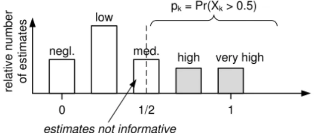
pk :=Pr[Xk >0.5]. (1)

Under this heuristic, the likelihood for the problem to jump over an edge of class k is determined by how much mass the experts put on the event of an infection. Continuing the above example with the qualitative scale (low < medium

< high) for the likelihoods, this would mean that, e.g., a “medium” assessment contributes no information, as it assigns mass to the exact center, or equivalently, puts equal mass on both events, to infect or not infect a node. This is (at least intuitively) meaningful, as infections are more frequent in the simulation if more experts consider an edge as being a likely infection path. Conversely, if experts rate the chance of an infection over an edge of class k rather low, then the simulation adheres to this expected behavior. Figure 1 shows an abstract example of a distribution that is constructed from several experts rating an edge of class k on a five part scale “negligible/low/medium/high/major”. The values of the grayish highlighted bars are merely summed up to give the sought likelihoodpk.

The likelihood used for the simulation according to the above formula is the mass located to the right of the center. This rule offers the additional appeal of being somewhat robust against outliers, which in case of risk expertise elicitation would correspond to extreme risk aversion or extreme will-ingness to take risks. Experts that fall into either of these classes would not affect the 50%-quantile (that pk according to equation (1) basically is).

An alternative yet most likely computationally infeasible approach would be averaging over all different configurations of edge likelihoods, which are available from the total set of expert opinions. It is easy to imagine that – if a discrete scale

is used – the number of simulations grows likeΩ(nm_{), where}

mis the number of edge classes, andnis the minimal number of different estimates forpk per classk. Aggregating all these simulation outputs into a single weighted sum (with weights determined by the relative fraction of how often a particular configuration appears in the overall set) is also only feasible under discrete estimates. If the assessment is on a continuous scale (unlikely but possible in practice), then things become even more involved and unclear in how to define them properly.

C. A Pandemic Criterion from Percolation Theory

The question of primary interest is whether or not an infection stays local or evolves unboundedly across the net-work, such that every part of the system is ultimately reached. Running the simulation algorithm from section II-A multiple times to see where the infection is leading to, takes a lot of time and effort. Thus, a more direct answer to the question is required.

Alas, a naive use of a shortest-path algorithm to compute the most likely infection path fromv0to all other nodes inV,

is flawed, since this would return only oneamong (in general exponentially)manypossible ways over which an infection can hit a node. Thus, a more sophisticated model is needed, which percolation theory provides.

Since the formal proofs are messy and involved (see [33] for full details), the following description stays at an intuitive and high level.

Existing percolation models for spread of failures or epi-demics hardly take into account diversity among different connections but assume uniform probability of failure [34] (an approach that distinguishes at least directed from undirected connections can be found in [8]). Based on the model as described in section II, especially the different probabilities

pi for each edge classi, the structure of the infected part of the network can be determined using probability generating functions (see e.g. [35]). Intuitively, these help answering the following question:

How big is the impact of an error, i.e., what is the expected number of infected nodes due to failure of a component?

The “size” of the impact is herein taken as the average number of infected nodes (taken as the limit over a hypo-thetical infinitude of independent simulations). A pandemic outbreak is then nothing else than an unbounded average number of infected nodes. The subsequently stated criterion to predict this pandemic is based on this understanding:

Definition 2.1 (Pandemic Outbreak): A pandemic in a graph G occurs if the expected number of affected nodes is unbounded.

For both failure of a node as well as of an edge of class

i, a linear equation system in the expected number of infected nodes can be obtained. The coefficient matrix is therein fully determined by the graph topology (specifically the probability

qk for an edge of type k to exist in the network), and the probabilitypk for an edge of typekto transport the problem. The scope of the outbreak is governed by these probabilities,

(a) Situation after 5 time units (b) Situation after 10 time units

Fig. 2: Bounded Epidemic (Condition (2) satisfied)

and whether or not a pandemic occurs can be decided upon knowing these quantities.

If the network is described through an Erd˝os-R´enyi model [36], the equation system is directly solvable and yields a particularly simple relation between the network properties and a possible pandemic:

Theorem 2.1: Let a network ofnnodes withmclasses of edges be described through a Erd˝os-R´enyi model, in which an edge of classiexists with probabilityqi. Furthermore, let each class i have probability pi to let an error propagate over an edge of this kind. If

1−np1q1−. . .−npmqm>0, (2)

thenno pandemic (according to def. 2.1) will occur.

The theorem can be illustrated using the simulation algo-rithm of section II-A: Assume the network to consist of 20 nodes with 3 different classes of connections, shown in red, green and black (cf. Fig. 2 and Fig. 3). Let the probabilities for an edge to exist in each class be q = (0.1,0.1,0.1) and let the error propagate over each class with likelihoods

p = (0.1,0.2,0.05). Then, the hypothesis of 2.1 is satisfied and a rather limited fraction of nodes is expected to fail. Indeed, the simulation results shown in Figure 2 display only one infection (node colored red) having occurred after ten time units after the initial incident. On the contrary, if the probabilities for existence of a link are q = (0.1,0.4,0.25) and those for an error propagation arep= (0.1,0.3,0.25), then the “anti-pandemic” condition in theorem 2.1 is violated, and a pandemic is expected. The simulation indeed confirms this behavior, as Figure 2 shows only 3 of the 20 nodes remaining healthy 10 time steps after the outbreak (the other 17 nodes are all red).

III. VISUALIZATION BYHEAT-MAPS AND GEO-REFERENCES

In its plain form, the simulation delivers a concrete scenario of infections, and the percolation epidemics criterion judges the (un)boundedness of the average number of infections. Both pieces of information can be made much more comprehensi-ble by a visualization technique, which adds the geographic location to each node, and – using color codes – indicates the likelihood of a node becoming infected as the relative frequency of its red-coloring over many simulations of the outbreak. Speaking percolation language, a pandemic outbreak

(a) Situation after 5 time units (b) Situation after 10 time units

Fig. 3: Pandemic Outbreak (Condition (2) violated)

will then become visible by a giant red component in the infrastructure, while a locally bounded epidemic will appear as a smaller bounded cluster in the network infrastructure.

For the general problem of incident propagation, it is useful to consider the way in which infrastructures can be modeled beyond pure physical connections. This is a standard step to gain an understanding of the infrastructure, and it can have a second use in identifying the proper edge classes to set up the percolation model as described in section II. Usually, such modeling is aided by a good visualization, which also can have a double use, namely, to set up the model and to visualize the results.

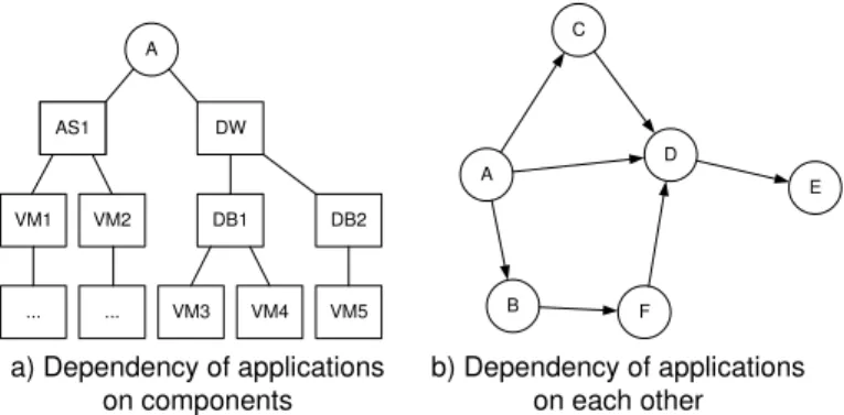
To get started with the model, [32] proposes a modularized approach that can be adopted here too: This process starts with an identification of physical components and applications, and interdependencies therein. Figure 4a displays an example of such a dependency model, in which an application A depends on several subcomponents, e.g., an application server (AS1), a data warehouse (DW), which itself relies on (two) databases DB1, DB2, and components are virtualized (represented by virtual machine nodes VM1, . . . , VM5, which in turn run on physical servers, etc.

Figure 4b represents a higher-level view that is restricted basically to interdependencies between applications. Thus, in distinguishing dependencies between components from those between applications, two edge classes for the percolation anal-ysis have already been identified. The resulting infrastructure model is nothing else than a weighted directed graph that captures dependencies of physical components and/or applica-tions on one another. More precisely, nodes are components or applications and edges are relationships between components, each of which falls into a specific edge class (determined by the type of dependency), and has a specific behavior in error propagation. In this logical view, model components-to-components relations, as well as components-to-application and applications-to-application-relationships, by defining the respective edge classes. The graph representation is in no way restricted in its visual elements, so the model itself can use boxes and circles to distinguish components from applications, while both are being abstracted to simple “nodes” in the graph model Gfor the percolation.

On the so-obtained graphical dependency model, the pan-demic criterion (theorem 2.1) can be invoked to obtain a first (initial) risk estimate. For a more detailed picture, the proposed

AS1 DW AS1

VM1 VM2 DB1 DB2

... VM4

... VM3 VM5

A

A C

D

B F

E

a) Dependency of applications on components

b) Dependency of applications on each other

Fig. 4: Dependency Model – Example

simulation can be executed, with its results fed back into the visualization technique of [32], to get the sought “zoomable” information and visualization system. The visualization is nothing else than the initial dependency model, only being aug-mented by color codes to indicate neuralgic spots. A decision maker can then coarsen or refine the graph by clustering nodes or dissolving cluster-nodes to display more or less details. For example, one can (un)hide the physical dependencies below application A from the higher-level application dependency graph in Figure 4b. Also it is easy to augment nodes with meta information, such as the node type, the geographical location, the likelihood of an infection, and whatever else is relevant. This is the typical case for visualizations as being used in a security operation center, as they are used by governments or agencies to supervise the security situation in IT infrastructures (e.g., a local intranet, a critical infrastructure, etc.).

An important part of the meta-information is directly ob-tained from the percolation simulation, and meta-information about the infrastructure as a whole can be gathered from the pandemic criterion as given in section II-C. For example, imag-ine that a number of independent simulations are done, then the outcome of each one (specific infection or error propagation scenario) may be different per run. Simply counting the relative number of times that application A has been infected by the simulated incident, approximates the likelihood for A to be eventually in trouble. This likelihood can be displayed using a color indicator, as shown in Figure 5. That is, instead of coloring a node green or red as in the simulation, the analysis would now assign any color between purple (high likelihood of a problem) until green (low likelihood of a problem), to graphically visualize which parts of an infrastructure are critical, vulnerable, etc.

The resulting picture is called a heat-map, and could look like figure 5. In this image, the circles represent applications (only), and the color codes indicate the vulnerability of an application to running into trouble. In the simplified picture shown in figure 5, application A as being infected by malware may also infect C with some likelihood, but D remains somewhat secure, although E is affected with high probability again. This simplified view does not explain this effect, which, however, may be due to the error propagating from A to E over some edges that belong to a class that is hidden in this view.

In general, by displaying different edge classes, different pictures arise, and explanations for vulnerabilities can be found from the graphical model almost directly.

A C

D

B F

E

Fig. 5: Heatmap example

In a second step of the visualization, the risk manager can look at the meta-information attached to the nodes in the heatmap, so as to change the heatmap according to what the decision maker are currently interested in. For example:

• Layers of security: these determine the depth of in-formation details. In the first layer, applications and their relations are presented (as one edge class). In a second layer, components that applications depend on can be represented (another edge class), and so on. Thus, the security layers may directly correspond to edge classes. Depending on what edge classes are being displayed, the picture may change (see figure 6).

Fig. 6: Showing different layers

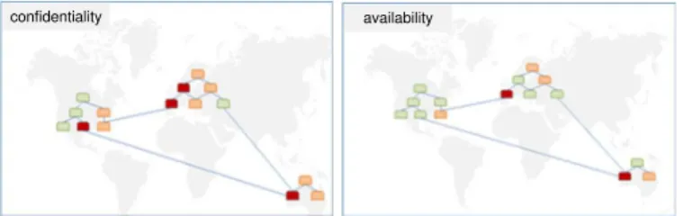
• Protective target: the simulation/percolation may refer to different security targets, which amounts to assign-ing different probabilities to the existassign-ing edge classes. For example, if the security goal is integrity, then inconsistencies in the data delivered by application A may cause subsequent errors in application B as well (as A delivers data to B). If the protective target is availability, then an outage of application A may cause much less troubles with application B. The respective heatmaps may look very different, and – combined with geographical data – directly point to the most likely problems (see figure 7).

• Different filters can be used to omit parts/details from the picture if they are not relevant. These filters could concern the infection grade (to show only highly vulnerable spots) or to restrict the view on a specific country or subsidiary of an enterprise. For example, an important filter concerns the connectivity of a node, to see which nodes are easy to isolate or repair. Such filters are useful to define remediation plans, if an epidemic (or pandemic) is indicated.

confidentiality availability

Fig. 7: Showing different protective targets

IV. CONCLUSION

Percolation offers a simple, intuitive and powerful model of epidemics spreading in networks, which is particularly applicable to risk propagation. A current limitation of this model is its ignorance of recovery or healing effects, which may take place in long run simulations or even when advanced persistent threats (APTs) are being mounted (when malware that has not yet become active is removed by coincidence or upon detection).

For a decision maker and security expert, both not con-cerned with the details of the theory but how to apply its results in practice, the method offers several appealing features: first, it can easily deal with uncertainty and ambiguity in the model parameters. Although the model’s outcome is only as good as its input, the full variety of methods to deal with uncertainty is available to aggregate diverging opinions into a justified model parameter. In this context, equation (1) is robust against outliers, i.e., unusual/uninformed risk assessments, but a Bayesian estimate would be equally possible. Second, the theory as such provides a direct answer to a frequent direct question, i.e., “whether or not the system is going to be in trouble”. If the answer to the latter is positive, then the visualization technique (as sketched in section III) allows to dig into the simulation data (as obtained by the simple algorithm in section II-A), to let a decision maker “zoom-into” the picture to see different scenarios of incident propagation, to manually and informedly refine her/his opinion about what needs to be done.

ACKNOWLEDGMENT

This work was partially supported by the European Com-mission’s Project No. 608090, HyRiM (Hybrid Risk Manage-ment for Utility Networks) under the 7th Framework Pro-gramme (FP7-SEC-2013-1).

REFERENCES

[1] D. Duffie, S. Malamud, and G. Manso, “Information percolation with equilibrium search dynamics,”Econometrica, vol. 77, no. 5, pp. 1513– 1574, September 2009.

[2] ——, “Information percolation in segmented markets,” National Bureau of Economic Research, Tech. Rep., 2011, working Paper 17295. [3] ISO International Organization for Standardization, ISO 31000:2009

Risk management – Principles and guidelines. Geneva, Switzerland: ISO International Organization for Standardization, 2009.

[4] ——,ISO 31010:2009 Risk management – Risk assessment techniques. Geneva, Switzerland: ISO International Organization for Standardiza-tion, 2009.

[5] ——, ISO/IEC 27005:2011 Information technology – Security tech-niques – Information security risk management. Geneva, Switzerland: ISO International Organization for Standardization, 2011.

[6] L. M. Sander, C. P. Warren, I. M. Sokolov, C. Simon, and J. Koopman, “Percolation on heterogeneous networks as a model for epidemics,”

Mathematical Bioosciences, vol. 180, pp. 293–305, 2002.

[7] M. E. J. Newman, “The spread of epidemic disease on networks,”

Physical Review E, vol. 66, 016128, 2002.

[8] L. A. Meyers, M. E. J. Newman, and B. Pourbohloul, “Predicting epi-demics on directed contact networks,”Journal of Theoretical Biology, vol. 240, no. 3, pp. 400–418, 2006.

[9] E. Kenah and M. Robins, “Second look at spread of epidemics on networks,”Physical Review E, vol. 76, 036113, 2007.

[10] J. C. Miller, “Bounding the size and probability of epidemics on networks,”Applied Probability Trust, vol. 45, pp. 498–512, 2008. [11] O. Diekmann, J. A. P. Heesterbeek, and M. G. Roberts, “The

construc-tion of next-generaconstruc-tion matrices for compartmental epidemic models,”

Journal of the Royal Society Interface, vol. 47, no. 7, 2010. [12] M. E. J. Newman and C. R. Ferrario, “Interacting epidemics and

coinfection on contact networks,”PLoS ONE, vol. 8, no. 8, 2013. [13] M. Salath´e and J. H. Jones, “Dynamics and control of diseases in

networks with community structure,”PLoS Comput Biol, vol. 4, no. 6, 2010.

[14] M. E. J. Newman and C. R. Ferrario, “Competing epidemics on complex networks,”Physical Review E, vol. 84, 036106, 2011.

[15] T. Tassier,The Economics of Epidemiology. Springer, 2013. [16] G. Grimmett,Percolation. Springer, 1989.

[17] D. S. Callaway, M. E. J. Newman, S. H. Strogatz, and D. J. Watts, “Network robustness and fragility: Percolation on random graphs,”

Physical Review Letters, vol. 85, no. 25, 2000.

[18] R. Cohen, D. ben Avraham, and S. Havlin, “Percolation critical ex-ponents in scale-free networks,”Physical Review E, vol. 66, 036113, 2002.

[19] N. Schwartz, R. Cohen, D. ben Avraham, A.-L. Barabasi, and S. Havlin, “Percolation in directed scale-free networks,”Physical Review E, vol. 66, 015104, 2002.

[20] Bundesamt f¨ur Sicherheit in der Informationstechnik, “BSI-Standard 100-2: IT-Grundschutz Methodology,” https://www.bsi.bund.de/cln 156/ContentBSI/grundschutz/intl/intl.html, May 2008, version 2.0, english.

[21] S. Poggi, F. Neri, V. Deytieux, A. Bates, W. Otten, C. Gilligan, and D. Bailey, “Percolation-based risk index for pathogen invasion: appli-cation to soilborne disease in propagation systems,”Psychopathology, vol. 103, no. 10, pp. 1012–9, 2013.

[22] S. Karnouskos, “Stuxnet worm impact on industrial cyber-physical system security,” in 37th Annual Conference of the IEEE Industrial Electronics Society (IECON 2011), Nov 2011, pp. 4490–4494. [23] A. Scarfo, “New security perspectives around BYOD,” inBroadband,

Wireless Computing, Communication and Applications (BWCCA), 2012 Seventh International Conference on, Nov 2012, pp. 446–451. [24] G. Thomson, “BYOD: enabling the chaos,”Network Security, pp. 5–8,

Feb 2012.

[25] B. Morrow, “BYOD security challenges: control and protect your most sensitive data,”Network Security, pp. 5–8, Dez 2012.

[26] Logicalis, BYOD: an emerging market trend in more ways than one, 2012.

[27] D. D. Dudenhoeffer and R. Permann, M.R. und Boring, “Decision consequence in complex environments: Visualizing decision impact,” in Proceeding of Sharing Solutions for Emergencies and Hazardous Environments. American Nuclear Society Joint Topical Meeting: 9th Emergency Preparedness and Response/11th Robotics and Remote Systems for Hazardous Environments, 2006.

[28] D. D. Dudenhoeffer and M. Permann, M. R. und Manic, “CIMS: A framework for infrastructure interdependency modeling and analysis,” inProceedings of the 2006 Winter Simulation Conference, New Jersey, 2006.

[29] US Government, “Executive order, 13010. critical infrastructure protec-tion,” pp. 3747–3750, 1996, federal Register.

[30] S. Rinaldi, J. Peerenboom, and T. Kelly, “Identifying, understanding, and analyzing critical infrastructure interdependencies,”IEEE Control Systems Magazine, pp. 11–25, 2001.

[31] P. Pederson, D. D. Dudenhoeffer, S. Hartley, and M. R. Permann, “Critical infrastructure interdependency modeling: A survey of U.S. and international research,” Idaho National Laboratory, Tech. Rep., 2006, INL/EXT-06-11464.

[32] A. Beck, M. Trojahn, and F. Ortmeier, “Security risk assessment framework,” in DACH Security 2013, P. Schartner and P. Trommler, Eds. syssec, 2013, pp. 69–80.

[33] S. K¨onig, S. Rass, and S. Schauer, “Report on Definition and Cate-gorisation of Hybrid Risk Metrics,” HyRiM Consortium, FP7 Project no. 608090 Hybrid Risk Management for Utility Networks, Tech. Rep. D1.2, 2015.

[34] R. Cohen, K. Erez, D. ben Avraham, and S. Havlin, “Resilience of the internet to random breakdowns,”Physical Review Letters, vol. 85, no. 21, 2000.

[35] M. E. J. Newman, S. H. Strogatz, and D. J. Watts, “Random graphs with arbitrary degree distributions and their applications,”Physical Review E, vol. 64, 026118, 2001.

[36] P. Erd˝os and A. R´enyi, “On random graphs,”Publicationes Mathemat-icae, vol. 6, pp. 290–297, 1959.