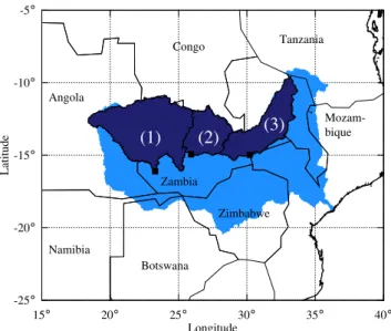
Hydrological real-time modelling in the Zambezi river basin using satellite-based soil moisture and rainfall data
Texto
Imagem
Documentos relacionados
and Wood, E.: The assimilation of remotely sensed soil brightness temperature im- agery into a land surface model using ensemble Kalman filtering: a case study based on
“Impact of rainfall spatial distribution on rainfall-runoff modelling efficiency and initial soil moisture conditions estimation” published in Nat.. Hazards
It is based on the hydrological soil group, Land use/Land cover and daily rainfall data daily runoff depth which were estimated by MNRCS-CN method using
Climate information based streamflow and rainfall forecasts for Huai River basin using hierarchical Bayesian modeling..
Using satellite-based MODIS data (land surface temperature data, EVI, etc.), and ground-based on-site soil moisture data and meteorological data (air tempera- ture, relative
To assess the usefulness of coarse resolution soil moisture data for catchment scale modelling, scatterometer derived soil moisture data was compared to hydrometric measure-
relative soil moisture content is for all the rainfall scenarios more or less the same. The temporal variance in soil moisture is overestimated when using rainfall information
Based on rainfall, soil evaporation, tran- spiration, runo ff and soil moisture measurements, a water balance model has been developed to simulate soil moisture variations over
