Global distributions of CO<sub>2</sub> volume mixing ratio in the middle and upper atmosphere from daytime MIPAS high-resolution spectra

(1)

www.atmos-meas-tech.net/9/6081/2016/ doi:10.5194/amt-9-6081-2016

Global distributions of CO

2

volume mixing ratio in the middle and

upper atmosphere from daytime MIPAS high-resolution spectra

Á. Aythami Jurado-Navarro1_{, Manuel López-Puertas}1_{, Bernd Funke}1_{, Maya García-Comas}1_{, Angela Gardini}1_,

Francisco González-Galindo1_{, Gabriele P. Stiller}2_{, Thomas von Clarmann}2_{, Udo Grabowski}2_{, and Andrea Linden}2

1_{Instituto de Astrofísica de Andalucía, CSIC, Granada, Spain}

2_{Institute for Meteorology and Climate Research (IMK-ASF), Karlsruhe Institute of Technology (KIT), Karlsruhe, Germany}

Correspondence to:Manuel López-Puertas ([email protected])

Received: 1 March 2016 – Published in Atmos. Meas. Tech. Discuss.: 15 March 2016 Revised: 30 November 2016 – Accepted: 4 December 2016 – Published: 20 December 2016

Abstract.Global distributions of the CO2vmr (volume

mix-ing ratio) in the mesosphere and lower thermosphere (from 70 up to∼140 km) have been derived from high-resolution

limb emission daytime MIPAS (Michelson Interferometer for Passive Atmospheric Sounding) spectra in the 4.3 µm re-gion. This is the first time that the CO2vmr has been

re-trieved in the 120–140 km range. The data set spans from January 2005 to March 2012. The retrieval of CO2has been

performed jointly with the elevation pointing of the line of sight (LOS) by using a non-local thermodynamic equilib-rium (non-LTE) retrieval scheme. The non-LTE model in-corporates the new vibrational–vibrational and vibrational– translational collisional rates recently derived from the MI-PAS spectra by Jurado-Navarro et al. (2015). It also takes ad-vantage of simultaneous MIPAS measurements of other at-mospheric parameters (retrieved in previous steps), such as the kinetic temperature (derived up to ∼100 km from the

CO2 15 µm region of MIPAS spectra and from 100 up to

170 km from the NO 5.3 µm emission of the same MIPAS spectra) and the O3measurements (up to∼100 km). The

lat-ter is very important for calculations of the non-LTE popu-lations because it strongly constrains the O(3_P_{) and O(}1_D₎

concentrations below∼100 km. The estimated precision of

the retrieved CO2vmr profiles varies with altitude ranging

from ∼1 % below 90 km to 5 % around 120 km and larger

than 10 % above 130 km. There are some latitudinal and sea-sonal variations of the precision, which are mainly driven by the solar illumination conditions. The retrieved CO2

pro-files have a vertical resolution of about 5–7 km below 120 km and between 10 and 20 km at 120–140 km. We have shown that the inclusion of the LOS as joint fit parameter improves

the retrieval of CO2, allowing for a clear discrimination

be-tween the information on CO2 concentration and the LOS

and also leading to significantly smaller systematic errors. The retrieved CO2 has an improved accuracy because of

the new rate coefficients recently derived from MIPAS and the simultaneous MIPAS measurements of other key atmo-spheric parameters (retrieved in previous steps) needed for non-LTE modelling like kinetic temperature and O3

concen-tration. The major systematic error source is the uncertainty of the pressure/temperature profiles, inducing errors at mid-latitude conditions of up to 15 % above 100 km (20 % for polar summer) and of∼5 % around 80 km. The errors due

to uncertainties in the O(1_D_{) and O(}3_P_{) profiles are within}

3–4 % in the 100–120 km region, and those due to uncer-tainties in the gain calibration and in the near-infrared so-lar flux are within∼2 % at all altitudes. The retrieved CO₂

shows the major features expected and predicted by general circulation models. In particular, its abrupt decline above 80– 90 km and the seasonal change of the latitudinal distribution, with higher CO2 abundances in polar summer from 70 up

to∼95 km and lower CO₂vmr in the polar winter. Above ∼95 km, CO₂is more abundant in the polar winter than at

the midlatitudes and polar summer regions, caused by the re-versal of the mean circulation in that altitude region. Also, the solstice seasonal distribution, with a significant pole-to-pole CO2 gradient, lasts about 2.5 months in each

(2)

100 1000 Regularization strength (no units) 40

60 80 100 120 140

Altitude [km]

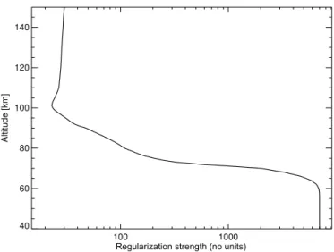
Figure 1. Regularization strength used in the retrieval of the

CO₂vmr.

1 Introduction

Carbon dioxide, CO2, plays a major role in the radiative

en-ergy budget of the atmosphere. Its 15 µm band is the major infrared cooling below around 120 km, and it also causes a significant heating of the upper mesosphere by the absorption of solar radiation in its near-infrared bands (see e.g. López-Puertas and Taylor, 2001). Hence, CO2 has a critical effect

on the atmospheric temperature structure and therefore it is very important to know its global (altitude and latitude) dis-tribution accurately (see e.g. Garcia et al., 2014).

CO2 was first measured in the upper atmosphere by

in situ measurements carried out by rocket-borne mass spectrometers (Offermann and Grossmann, 1973; Trinks et al., 1978; Trinks and Fricke, 1978). The Spectral In-frared Rocket Experiment (SPIRE) measured its 15 µm non-LTE (non-local thermodynamic equilibrium) emission (Stair et al., 1985). The Improved Stratospheric and Mesospheric Sounder (ISAMS) aboard the Upper Atmosphere Research Satellite (UARS) carried out 4.6 µm global measurements performing simultaneous measurements of temperature and pressure up to 80 km (López-Puertas et al., 1998; Zaragoza et al., 2000). CO2 number densities were retrieved from

daytime limb radiance measured by the Cryogenic Infrared Spectrometers and Telescopes for the Atmosphere (CRISTA) measurements in the 60–130 km region (Kaufmann et al., 2002). For a complete review of early measurements until 2000 see López-Puertas et al. (2000). More recently, two satellite CO2data sets have been made available. The Fourier

transform spectrometer on the Canadian Atmospheric Chem-istry Experiment (ACE-FTS) has measured the CO2vmr in

the mesosphere and lower thermosphere (70 to 120 km) by using the solar occultation technique. This approach has the advantage of being free from non-LTE effects (and the er-rors associated to the knowledge of the non-LTE population

of the emitting states) but provides limited latitudinal cover-age (Beagley et al., 2010). Almost simultaneously with ACE, the Sounding of the Atmosphere using Broadband Emis-sion Radiometry (SABER), on board the NASA Thermo-sphere IonoThermo-sphere Energetics and Dynamics (TIMED), has been measuring the atmospheric limb radiance in the 15 and 4.3 µm channels. Rezac et al. (2015) applied a simultaneous temperature–CO2vmr retrieval to these measurements and

produced a long (13-year) database of CO2in the middle and

upper atmosphere.

In this paper we describe the inversion of CO2vmr from

MIPAS (Michelson Interferometer for Passive Atmospheric Sounding) high-resolution daytime limb emission spectra in the 4.3 µm region. MIPAS is able to discriminate the contri-butions of the many CO2bands that give rise to the 4.3 µm

atmospheric emission; thus in a previous work it allowed us to obtain a more accurate knowledge of the CO2 non-LTE

processes that control the population of the emitting levels near 4.3 µm (Jurado-Navarro et al., 2015). In that work the large impact of the new collisional rates on the limb atmo-spheric radiance near 4.3 µm was demonstrated (see Figs. 11 and 12 in that paper). Several tests performed in that study have also shown a substantial effect on the retrieved CO2.

Therefore, the use of those retrieved collisional rates allowed us to retrieve CO2with a much better accuracy in the present

work than in previous limb emission measurements. In addi-tion, the high spectral resolution allows for a proper selection of the spectral points (optically thin and moderate points of the lines of the bands) containing the largest amount of in-formation at different tangent heights, which constrains the retrieval better than an integral wideband radiance measure-ment.

In Sect. 2 we describe the MIPAS instrument and the mea-surements, and in Sect. 3 the retrieval method and the set-up. The advantages of using the CO2-LOS (line of sight) joint

retrieval are discussed in Sect. 4. In Sect. 5 we discuss the major characteristics of the retrieved CO2vmr and the error

analysis. Finally, in Sect. 6 we provide and discuss a monthly climatology based on the data retrieved in 2010 and 2011. A validation and comparison of MIPAS CO2 data with ACE

and SABER measurements, as well as with Whole Atmo-sphere Community Climate Model (WACCM) simulations, are to be presented in a future paper.

2 MIPAS observations

The MIPAS instrument is a mid-infrared limb emission spec-trometer designed and operated for measurements of atmo-spheric trace species from space (Fischer et al., 2008). It was part of the payload of Envisat launched on 1 March 2002 with a sun-synchronous polar orbit of 98.55◦_{N inclination and an}

(3)

profiles of spectra. The instrument’s field-of-view is 30 km in the horizontal and approximately 3 km in the vertical direc-tion. From January 2005 until the end of Envisat’s operations on 8 April 2012, MIPAS measured at a optimized spectral resolution of 0.0625 cm−1_.

The MIPAS instrument sounded the middle and upper mospheres in three measurements modes: MA (middle at-mosphere), UA (upper atmosphere) and NLC (noctilucent clouds). The UA mode, scanning the limb from 42 to 172 km, was specifically devised for measuring the thermospheric temperature and CO2 and NO abundances. In the MA and

NLC modes, MIPAS took spectra up to 102 km only. How-ever, since many lines of the CO2fundamental band (those

with a larger signal) are still optically thick at this tangent height and above, they reduce the sensitivity to the retrieved CO2below 102 km. Thus, having measurements above that

altitude are very important for retrieving the CO2in the

opti-cally thin regime and hence better constraining the CO2vmr

below. As a consequence, the retrieval set-up and the de-rived CO2 presented here, data version v5r_CO2_622,

cor-respond to the UA observation mode. Only daytime data were used since the night-time observations are very noisy and non-LTE processes are not known that accurately. Note that the three MIPAS modes have very similar temporal and latitudinal coverages. Hence the retrieval of CO2 from the

MA and NLC modes would not significantly extend the coverage of the CO2 UA database. The limb vertical

sam-pling of the UA mode is 5 km from 172 km down to 102 km and 3 km below, recording a rear viewing sequence of 35 spectra every 63 s. Its along-track horizontal sampling is of about 515 km (De Laurentis, 2005; Oelhaf, 2008). Version V5 (5.02/5.06) of the L1b calibrated and geo-located spec-tra processed by the European Space Agency (ESA; Perron et al., 2010; Raspollini et al., 2010) were used here for the retrieval of CO2 and for all other parameters used in its

re-trieval, namely, pressure/temperature and ozone.

3 The retrieval method and its set-up

Carbon dioxide vmr profiles together with the elevation pointing of the line of sight (LOS) are retrieved using the MI-PAS level 2 processor developed and operated by the Institute of Meteorology and Climate Research (IMK) together with the Instituto de Astrofísica de Andalucía (IAA). The proces-sor is based on a constrained non-linear least squares algo-rithm with Levenberg–Marquardt damping (von Clarmann et al., 2003). Its extension to retrievals with consideration of non-LTE (i.e. CO, NO and NO2) is described by Funke

et al. (2001). Non-LTE vibrational populations of CO2 are

modelled with the Generic RAdiative traNsfer AnD non-LTE population Algorithm (GRANADA; Funke et al., 2012; see more details below) within each iteration of the retrieval.

Following the scheme described by von Clarmann et al. (2003), the following retrieval equation is used:

xi+1=xi+ h

KT_S−1

y K+R+λI i−1

× n

KTS−1

y [ymeas−y(xi)] −R(xi−xa) o

, (1)

whereK is themmax×nmax Jacobian, containing the

par-tial derivatives of allmmaxsimulated measurementsy(x) un-der consiun-deration with respect to all unknown parametersx, superscriptT denotes a transposed matrix, x is the nmax–

dimensional vector of unknown parameters and xa is the related a priori information. The term y_meas is the mmax

-dimensional vector of measurements under consideration, y(xi)is the forward modelled spectrum using parametersxi

from thei-th step of iteration.Ris ann_max×n_max

regulariza-tion matrix, andSyis themmax×mmaxcovariance matrix of the measurement. The termλI(tuning scalar times the unity

matrix) dampens the step widthxi+1−xi, bends its direc-tion toward the direcdirec-tion of the steepest descent of the cost function in the parameter space and prevents a single itera-tion from causing a jump of parametersxbeyond the linear domain around the current guessxi (Levenberg, 1944; Mar-quardt, 1963).

In our case, the column vectorx contains the CO2

pro-file (103 elements), the LOS propro-file (23 elements) and the radiance offset (17 elements, one per each microwindow). The a priori profile,xa, for CO2is taken from monthly zonal

means of the Whole Atmosphere Community Climate Model with specified dynamics (SD-WACCM) simulations span-ning over the time period of the measurements (Garcia et al., 2014). SD-WACCM is constrained with output from NASA’s Modern-Era Retrospective Analysis (MERRA) (Rienecker et al., 2011) below approximately 1 hPa. Garcia et al. (2014) showed SD-WACCM simulations for Prandtl numbers (Pr) of 4 (standard) and 2, corresponding to lower and higher eddy diffusion coefficients respectively. Here we used the simu-lations forPr =2, which gives an overall better agreement with ACE CO and CO2and MIPAS CO (Garcia et al., 2014).

In this way we expect to have a faster convergence with no impact of the a priori profile since the CO2profile is

regular-ized by means of a Tikhonov-type first-order smoothing con-straint (Tikhonov, 1963; see below). The a priori profile for the elevation pointing of the line of sight (LOS) was taken from that retrieved from the 15 µm region (García-Comas et al., 2014).

Since in the target altitude range we use a smoothing constraint only, x is not pushed towards the a priori file but the latter constrains the shape of the resulting pro-file only. Sy is the covariance matrix characterizing the measurement noise. Due to apodization (Norton and Beer, 1976) this matrix contains off-diagonal elements.R is the constraint matrix. CO2 is constrained by a Tikhonov-type

(4)

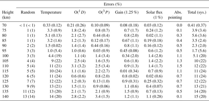
regu-Table 1.Errors of the CO₂vmr retrieved in this work for the midlatitude and polar summer (in parenthesis) conditions.

Errors (%)

Height Random Temperature O(1D) O(3P) Gain (1.25 %) Solar flux Abs. Total (sys.)

(km) (1 %) pointing

70 <1 (<1) 0.33 (0.12) 0.21 (0.26) 0.10 (0.09) 0.08 (0.18) 0.03 (0.12) 0.0 0.41 (0.37)

75 1 (1) 3.3 (0.9) 1.8 (2.4) 0.8 (0.7) 0.7 (1.7) 0.24 (1.2) 0.1 3.9 (3.4)

80 1 (1) 5.1 (0.13) 2.1 (2.7) 0.44 (0.4) 0.8 (2.0) 0.02 (1.1) 0.3 5.6 (3.6) 85 1 (1) 3.2 (1.6) 1.2 (1.3) 0.12 (0.17) 0.67 (1.1) 0.19 (0.18) 0.4 3.5 (2.4) 90 2 (2) 1.5 (0.02) 1.4 (1.4) 0.44 (0.16) 0.8 (1.1) 0.16 (0.12) 0.5 2.3 (2.0) 95 3 (3) 1.0 (5.4) 1.0 (0.6) 0.03 (0.9) 0.45 (0.08) 0.6 (1.2) 0.5 1.7 (5.6)

100 3 (3) 4.4 (19) 1.1 (4) 1.4 (3.4) 0.34 (2.0) 1.4 (2.8) 1.1 5.1 (20)

105 4 (4) 9 (22) 2.5 (4) 1.6 (3.5) 0.6 (1.8) 1.4 (2.2) 1.3 10 (22)

110 5 (4) 11 (21) 3.1 (3.2) 2.5 (3.4) 0.9 (1.3) 1.4 (1.7) 1.5 12 (22)

115 5 (5) 10 (24) 1.1 (1.6) 2.2 (2.7) 0.01 (0.34) 0.7 (0.9) 1.1 11 (24)

120 6 (5) 11 (24) 0.6 (0.6) 0.8 (2.0) 0.8 (0.02) 0.02 (0.6) 0.7 11 (24)

125 7 (7) 12 (22) 1.2 (0.3) 0.13 (1.0) 0.9 (0.31) 0.25 (0.32) 0.7 12 (22)

130 9 (9) 13 (21) 1.5 (1.1) 0.9 (0.06) 1.1 (0.6) 0.4 (0.07) 0.7 13 (21)

135 11 (12) 13 (20) 2.1 (1.7) 2.1 (0.9) 1.5 (0.9) 0.7 (0.13) 0.5 14 (20)

140 13 (14) 14 (20) 2.8 (2.2) 3.4 (1.5) 1.2 (1.1) 1.1 (0.28) 0.1 15 (20)

larization strength (von Clarmann et al., 2003). The regular-ization strength used here is shown in Fig. 1. Using those values, the constraint is optimized to obtain stable calcula-tions but with a precision high enough to allow for physically meaningful variations of the retrieved CO2abundance.

In addition, a strong diagonal constraint is added below 60 km in order to force the retrieved CO2to be close to the

well-known mixing ratio in the lower mesosphere. The en-tries correspond to the CO2a priori standard deviations of

∼0.5 %, in line with the errors of the CO₂vmr in the 5–

25 km region retrieved from ACE spectra (Foucher et al., 2011). Admittedly the combination of a smoothing constraint with a diagonal constraint at low altitudes also forces the re-sult towards the a priori profile in a certain altitude range above the threshold altitude where the diagonal constraint is active. This effect, however, dampens out very quickly (see e.g. Fig. 13a and b).

A Tikhonov first-order smoothing constraint is also used for the LOS retrieval, allowing for vertically coarse varia-tions of∼10–20 km of the tangent height spacing with

re-spect to the a priori profile. The LOS of the lowermost tan-gent height is strongly constrained to the a priori profile by means of a diagonal regularization. Typically, the obtained degrees of freedom for the LOS retrievals are about 2.

The Levenberg–Marquardt parameter λscales unityI. It

is zero by default and is set to positive values only when the retrieval is found to diverge. Linearity is checked explicitly along with the convergence test by comparing the modelled and linearly extrapolated spectrum. A retrieval counts as con-verged only if the linear prediction of then-1st step is close

enough to the explicit non-linear line-by-line calculation of thenth step. The stopping criterion is defined such that

con-vergence is reached for both the residual spectra and the

re-trieval parameter vector. The typical number of iterations is in the range of 3 to 6 and the convergence percentage is very high, about 99.4 %. For further details like the cost function we refer the reader to von Clarmann et al. (2003).

Besides the CO2vmr profile and LOS, a height- and

wave-number-independent radiance offset is also fitted jointly in the retrieval. Before starting the retrieval, the L1b spectra were corrected for the spectral shift. The temperature used in the retrieval was taken from that retrieved from the same MI-PAS spectra in the 15 µm region (García-Comas et al., 2014) below around 100 km, and that retrieved from the same MI-PAS spectra in the NO 5.3 µm emission (Bermejo-Pantaleón et al., 2011) from 100 up to 170 km. Both temperatures were merged in the 95–105 km region using a hyperbolic tangent function.

Pressure was implicitly determined by means of hydro-static equilibrium (total density was obtained from pressure and temperature and using the ideal gas law). The CO2

non-LTE model used in the non-non-LTE inversion is described in detail in Funke et al. (2012). However, the collisional co-efficients of many vibrational–vibrational and vibrational– translational processes were updated with the values re-trieved from MIPAS spectra as described in Jurado-Navarro et al. (2015). In addition, some of the collisional rates of that work were updated here because of the improvements in the calculation of the O(1D)concentration (see below) and

fur-ther refinements leading to smaller residual spectra. These updates include, first, the collisional rates of CO2(vd, v3)+ M⇌CO2(v_d′, v3−1)+ M with1vd=2−4 and M=N2, O2(processes 8a and 8b in Table 1 of Jurado-Navarro et al.,

2015) where the factorf has been changed from 0.82 to 0.7.

Secondly, the rate of N2(1)+O→N₂+O (process 10 in that

(5)

Figure 2.Jacobians in the 2316–2318 cm−1_{region for five different tangent altitudes (from bottom to top: 60, 72, 81, 90 and 102 km). Two}

panels are shown for each tangent altitude. Upper panel: normalized Jacobians where the dashed black line indicate the tangent altitude and the thick red line the micro-window extension. As a guide, the lower panels show the normalized radiance contributions for the most prominent CO₂lines: of the fundamental band (black), of the second hot 1001→1000 band (red), of the 0221→0220 band (green) and of

0201→0200 (orange).

(T /300)1.5cm3s−1 _and _f ₌_{1. This rate has been adapted}

from Whitson and McNeal (1977), taking the upper limit (within the error bars) at 300 K, and re-adjusting the tem-perature dependence, taking into account the measurements at higher temperatures. The values of this new rate at tem-peratures near 300 K are, however, similar to those used in Jurado-Navarro et al. (2015).

The non-LTE model also requires other input quantities that affect the non-LTE populations of the emitting states. In particular it requires the concentrations of O3, O(3P )and

O(1_D)_{. For ozone we used that retrieved from the same}

MI-PAS spectra in the 10 µm spectral region (Gil-López et al., 2005; Smith et al., 2013) below 100 km. The atomic oxy-gen and O(1_D_{) profiles below 100 km were generated from}

the O3retrieved from the same MIPAS spectra and the

pho-tochemical model described by Funke et al. (2012). Above 100 km, we took the atomic oxygen and O2 concentrations

from the NRLMSIS-00 model (Picone et al., 2002). The O(1_D)_{profile above 100 km has been updated from the}

pho-tochemical model by Funke et al. (2012), using the O2

(6)

2300 2320 2340 2360 2380

Wavenumber [cm-1]

60 80 100 120 140

Tangent height [km]

Figure 3.Occupation matrix used in the CO₂retrieval in the 4.3 µm

spectral region. Shaded regions represent the spectral regions se-lected and red dots the microwindow mask at each tangent height. The specific microwindows used in the retrieval are listed in the Supplement.

from O2photo-absorption that considers that, at wavelengths

shorter than ∼100 nm the O₂, ionization is the dominant

channel. We also included an overhead column above the top layer of the model proportional to the scale height of O2. This

O(1_D)_{photo-production has been compared with that}

calcu-lated for similar conditions by an independent UV radiative transfer model (González-Galindo et al., 2005; Garcia et al., 2014), finding differences smaller than 2 % at all altitudes. A variable solar spectral irradiance (SSI; Lean et al., 2005) was included in all the photochemical calculations in order to ac-count for solar UV variations along the MIPAS observation period.

The retrievals are performed from 42 up to 152 km, over a discrete altitude grid of 1 up to 50, 2 from 50 to 70, 1 from 70 to 80, 2 from 80 to 90, 1 from 90 to 110, 2.5 from 110 to 120 and 5 from 120 to 152 km. The selected grid provides balanced accuracy and efficiency. The forward calculations are performed at that grid but using an internal sub-grid to achieve very accurate radiances. The over-sampled retrieval grid, finer than the MIPAS vertical measurement grid (vary-ing from ≈3 below 100 km to≈5 km above that altitude),

makes the use of a regularization mandatory in order to ob-tain stable solutions. In the retrieval we use only the spectra taken in the tangent altitude range from 60 up to 142 km. The spectra above 142 km have a low signal-to-noise ratio and did not contain significant information. The numerical inte-gration of the signal over the vertical field-of-view (≈3 km

or ≈5 km) is done using seven pencil beams. The forward

model calculations along the line of sight (LOS) include gra-dients (along the LOS) in the non-LTE populations of the emitting levels caused by both kinetic temperature gradients as well as by different solar illumination conditions (variable solar zenith angle) along the LOS.

The retrievals are performed using selected spectral re-gions (micro-windows) in the 4.3 µm region in MIPAS chan-nel D (1820–2410 cm−1_{), which vary with tangent altitude,}

in order to optimize computation time and minimize system-atic errors (von Clarmann and Echle, 1998). In particular, er-ror propagation due to horizontal inhomogeneities have been minimized by excluding opaque spectral lines which are in-sensitive to tangent point conditions.

The selection of the spectral regions sensitive to the CO2

abundance is performed by calculating the 4.3 µm Jacobians and selecting those regions with a good local response. In this way, and thanks to the excellent MIPAS spectral reso-lution, we are able to select the spectral points sensitive to the CO2vmr, yet with a good signal-to-noise ratio, while

ex-cluding lines with non-local responses due to spectral satu-ration. We have selected 18 principal spectral regions within the 2300–2380 cm−1_{range, containing height-dependent}

mi-crowindows at 23 tangent heights from 60 up to 142 km. An illustration of the selection for a particular spectral region is shown in Fig. 2. At 60 km, the fundamental band line (black) shows a local response and hence it is selected in the micro-windows mask. On the contrary, the second hot lines (red and orange) do not give a local response (the Jacobians are much more extended in altitude or their maxima occur at altitudes well above the tangent height) and hence are not selected. They are, however, included in the microwindow mask for higher tangent heights, i.e. from 85 up to 102 km, where they have quite enough local sensitivity. In this example the fundamental band line is not selected from 72 to 90 km, al-though it again gives valuable information at 102 km. Around 100 km the information progressively comes from lines in the second hot band to those in the fundamental band.

In addition to the exclusion of spectral points with non-local response, we restricted the microwindows to the strongest lines (mainly fundamental and second hot bands lines that have the larger signal/noise ratio) at each altitude for reasons of computational efficiency. Additionally, spec-tral regions with interferences from the 636, 628, 627, 638 and 637 CO2isotopologues have been suppressed in order to

avoid systematic errors caused by the less accurate non-LTE modelling of these minor species, since the collisional rates affecting these energy levels were not retrieved by Jurado-Navarro et al. (2015).

The resulting selection of microwindows (occupation ma-trix) is shown in Fig. 3. The selected spectral points belong mainly to the lines of the fundamental band in the 60–72 and 102–142 km regions and of the second hot bands in the 75– 102 km region. More detailed information on the microwin-dows used in the retrieval at different altitudes is given in the Supplement.

The retrieval method was applied to all MIPAS UA day-time scans. We considered all scans with a solar zenith angle (SZA) smaller than 90◦ _{at the centre-of-scan tangent point.}

The change in the CO2non-LTE populations along the line of

(7)

0 100 200 300 400 Mixing ratio [ppmv] 60

80 100 120 140

Altitude [km] _{A priori}Retrieved

True

-40 -30 -20 -10 0 10

Relative difference [%]

0 100 200 300 400

Mixing ratio [ppmv] 60

80 100 120 140

True

0 20 40 60

0 100 200 300 400

80 100 120 140

True

-30 -20 -10 0 10 20

0 100 200 300 400

80 100 120 140

True

-20 0 20

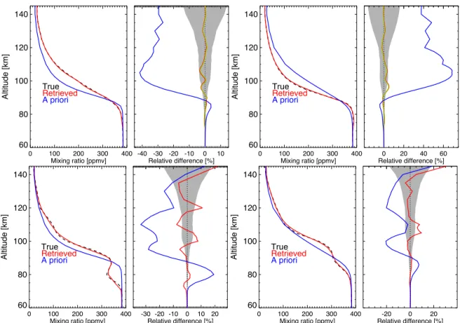
Figure 4.Sensitivity of the retrieved CO₂profile to the a priori CO₂profile for several conditions. Upper left panels: for a midlatitude true

profile and a polar summer a priori profile. Upper right panels: for a polar summer true profile and a midlatitude a priori profile. Lower left panels: for a true profile extremely low in the upper mesosphere as in Rezac et al. (2015) and a polar summer a priori profile. Lower right panels: for a true profile with an upper mesospheric wave-like perturbation and a midlatitude a priori profile. The relative differences true-retrieved profiles (right panels) are referred to the CO₂/LOS joint retrieval (red solid line) and to the single-parameter CO₂retrieval

(green line, hardly visible, shown only for the midlatitude and polar summer cases, upper row). The blue line is the a priori profile. The shaded area is the noise error of the retrieved profile. Note that the true-retrieved differences (red line) are within the noise error for nearly all altitudes and cases.

taken into account as described by Funke et al. (2009) for the case of CO.

4 Proof of concept of the CO2-LOS joint retrieval

In order to test the performance of the retrieval set-up we have applied it to synthetic spectra calculated for several atmospheric conditions using the Karlsruhe Optimized and Precise Radiative transfer Algorithm (KOPRA; Stiller et al., 2002) and the GRANADA non-LTE model. We investigate the sensitivity of the retrieval of CO2vmr to the CO2vmr and

LOS a priori profiles separately. In particular we are also in-terested in knowing if the retrieval yields reasonable results when the CO2and LOS a priori profiles are very different

from the actual atmospheric and observational conditions. The tested conditions include, first, the two most com-mon situations we expect to encounter in the retrievals: the midlatitude case, for which we have taken the April 45◦_N

daytime (SZA=44.5◦) reference atmosphere, and the

po-lar summer case for which we have taken the January 75◦_S

(SZA=58.7◦) reference atmosphere (Funke et al., 2012;

Jurado-Navarro et al., 2015). We have additionally consid-ered two other cases. One is the rather extreme CO2

pro-file that was found by Rezac et al. (2015) in the inversion of SABER radiances (see the top-right panel of their Fig. 12), with very low CO2vmr between 70 and 85 km and a

pro-nounced peak near 90 km. The other case was chosen to check if our algorithm would be able to retrieve the ex-pected effect of waves propagation on the CO2vmr profile

in the upper mesosphere and lower thermosphere. For this latter test, we looked at the variability of CO2vmr in the

WACCM model at all latitudes, longitudes and local times during a whole year of data co-located with MIPAS measure-ments and extracted the profile with the largest oscillation (see lower right panel of Fig. 4).

The CO2 a priori profiles for the four cases described

(8)

corre--0.03 -0.02 -0.01 0.00 0.01 0.02 0.03 LOS difference [km]

60 80 100 120 140

Altitude [km]

Figure 5. Sensitivity of the retrieved LOS (from the CO₂–LOS

joint retrieval) to the CO2a priori profile uncertainties for

midlati-tude (red) and polar summer (black) conditions. The lines show the retrieved–true LOS differences.

sponding to polar summer and, viceversa, for the true polar summer case we took as a priori profile the SD-WACCM pro-file corresponding to the midlatitudes. For the SABER-like CO2 true profile we choose the previous SD-WACCM

po-lar summer profile (corresponding to the seasonal conditions where it was found) and, for the wave-like CO2true profile,

we choose a typical smooth midlatitude profile.

Under midlatitude conditions, the retrieved CO2 profile

differs from the true profile by less than 2–3 % in the whole altitude region (upper left panels in Fig. 4). Compared to the difference with the a priori profile (up to 40 %), the agree-ment between the retrieved profile and the true one can be considered excellent. It is worth noting that the difference is smaller than the noise error at all altitudes. Regarding po-lar summer conditions, the differences between the retrieved and the true profiles are generally smaller than 2 % (the a pri-ori profile differs from the true profile up to 60 %) except at 95 to 110 km where the range is 2–4 % (upper right panels in Fig. 4). We also demonstrate that our algorithm would be able to retrieve unusual profiles such as those encountered by Rezac et al. (2015) in the SABER data (lower left pan-els in Fig. 4). Retrieved minus true differences are gener-ally smaller than 3 %. The only exceptions occur at altitudes where the true profile has abrupt gradients (note the blue line in the relative difference panel) where our algorithm, within its vertical resolution, is not able to fully recover them. Sim-ilarly, the lower right panels of Fig. 4 also shows that a wavy CO2profile as predicted by WACCM, with a wave amplitude

of about 20 %, would be fully recovered by our algorithm. We have also tested the effect of the a priori CO2 when

retrieving only the CO2vmr and keeping the LOS fixed, i.e.

with CO2as a single-parameter retrieval. The result is shown

by the green line in the upper panels of Fig. 4. We see that for both midlatitude and polar summer atmospheric conditions, the differences between the retrieved CO2with and without

the joint fit of LOS are only marginal. Very similar results are found for the other two cases (not shown). Also, the

inspec-0 100 200 300 400 Mixing ratio [ppmv] 60

80 100 120 140

Altitude [km]

Single retrieved Joint retrieved

True

-6 -4 -2 0 2 4 6 Relative difference [%]

0 100 200 300 400 Mixing ratio [ppmv] 60

80 100 120 140

Altitude [km]

Single retrieved Joint retrieved

True

-6 -4 -2 0 2 4 6 Relative difference [%] (a)

(b)

Figure 6. (a) Sensitivity of the retrieved CO₂ to LOS a priori

uncertainties for midlatitude conditions. The relative differences (retrieved–true) (right panel) are referred to the joint CO₂-LOS re-trieval (red solid line) and to the single-parameter CO2 retrieval

(green line).(b)As(a)but for polar summer conditions.

tion of the retrieved LOS in the joint fit case (Fig. 5) shows that the mapping of the CO2a priori uncertainties on the LOS

is very small (less than 20 m).

We also tested the impact of a perturbation of the LOS a priori information on the retrieved CO2. We applied a sine

function perturbation to the LOS with a value of 0 m at 60 and 142 km and a maximum of 200 m at 90 km. Above 90 km, the use of the perturbed a priori LOS profile in the CO2–LOS joint retrieval introduces deviations of the

re-trieved CO2from the true profile smaller than 1–2 %, while

differences are negligible below (see red line in Fig. 6a and b). On the other hand, the application of the perturbed LOS in the single-parameter CO2retrieval introduces a

sig-nificant systematic error of up to 3–4 % for the midlatitudes and an even larger error (up to 5 %) for polar summer above 70 km (see green line in Fig. 6a and b). In Sect. 5.2 we also discuss the effects of using the joint CO2-LOS or the CO2

(9)

-0.1 0.0 0.1 0.2 0.3 0.4 0.5 Averaging Kernel

60 80 100 120 140

Altitude [km]

-0.1 0.0 0.1 0.2 0.3 0.4 0.5 Averaging Kernel

60 80 100 120 140

Altitude [km]

(a)

(b)

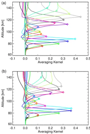
Figure 7. (a) Columns of the averaging kernel of the CO₂vmr

from the joint CO2-LOS retrieval for midlatitude conditions.(b)As

(a)but for polar summer conditions.

Therefore, these results give us confidence in the retrieval scheme and we conclude that the impact of a priori profile uncertainties on the retrieved CO2is very small, generally in

the.1–3 % range. Furthermore, fitting the LOS jointly was found to not degrade the retrieved CO2mixing ratios while

avoiding important systematic errors due to LOS uncertain-ties.

Figure 7a and b shows the columns of the averaging ker-nel (AK) of the CO2vmr from the joint CO2-LOS retrieval

at several altitudes for the most common cases of midlati-tude and polar summer conditions. Note that the magnimidlati-tude of the averaging kernel elements responds to both the instru-mental sampling (the coarser the sampling the smaller the AK elements) and the retrieval grid (the coarser the grid the larger the AK elements). Since both quantities vary with alti-tude, regions with different AK magnitudes occur. There are two clear regions with higher sensitivity, one ranging from around 75 to 95 km and another from ∼105 to 135 km. In

the lower region most of the information comes from the sec-ond hot bands (as discussed above) and, in the upper region, from the first, mainly fundamental 4.3 µm bands. There is a clear region in between where the sensitivity is smaller. It is also noticeable that, even after the careful selection of the microwindows, it is difficult to obtain information about the

CO2vmr in the lowermost latitudes, below around 70–75 km.

The averaging kernel column corresponding to the lower-most altitude shown in Fig. 7a and b, 72 km, maximizes a few kilometres above this altitude. It also has a negative tail above 120 km, caused by the strong regularization applied to the CO2 profile at its lower edge in conjunction with an

optically thick radiative transfer. The retrieval algorithm re-sponds to a positive perturbation of the CO2in the strongly

regularized profile range (below 70 km) with a reduction of the thermospheric CO2column (i.e. reduction of absorption).

Similar features are shown for the averaging kernel columns corresponding to altitudes below 72 km. The decrease of the vertical resolution above∼120 km is evident, with the

av-eraging kernels becoming wider, partially due to the coarser measurement sampling.

For a further check of the quality of the retrievals we in-spected the residual spectra at several tangent heights (see Fig. 8a and b). These figures show the residuals, not only at the spectral points used in the retrieval of CO2 (the

CO2 microwindows, red-shaded bands), but also at other

wave numbers, which informs us about the accuracy of the used collisional rates of the non-LTE model. In gen-eral, the residuals are very small, particularly in the CO2

microwindows. They still show, however, some systematic differences at wavelengths outside the CO2 microwindows

at lower tangent heights (72 km), but in the order of ±(1–

2) nW/(cm2_{sr cm}−1_{), which is only}_∼_{1 % of the signal. At}

smaller wave numbers (2280–2320 cm−1_{), a large fraction of}

these differences can be attributed to the 4.3 µm fundamental band of second isotopologue (636), for which the collisional rate with N2(1) was not retrieved by Jurado-Navarro et al.

(2015). At higher tangent heights the root mean square (rms) decreases, leading to even better simulations of the measure-ments, in particular, the radiance of the mentioned isotopic band.

The residuals for the polar summer latitudes (see Fig. 8b) are very similar to those for the midlatitudes, with rms very similar or even slightly smaller at lower tangent heights. At tangent heights of 92 and 102 km, we appreciate some systematic residuals which are more clear than at the mid-latitudes, though still very small. These residuals are most likely introduced by a systematic error in the kinetic temper-ature, distorting the rotational distribution, but could even be caused by rotational non-LTE.

It is important to remark that the residuals in the whole spectral range shown here, as a result of the inversion of CO2,

are nearly identical to those obtained in the retrieval of the collisional rates (compare Fig. 8a and b with Fig. 8 in Jurado-Navarro et al., 2015). Also note that the residuals in the CO2

(10)

2280 2300 2320 2340 2360 2380 2400 Wavenumber [cm-1_]

0 50 100 150

Radiance (nW cm

-2 sr -1 cm)

TH = 72 km

2280 2300 2320 2340 2360 2380 2400 Wavenumber [cm-1_]

-3 -2 -1 0 1 2

Residual

RMS = 0.596829

2280 2300 2320 2340 2360 2380 2400 Wavenumber [cm-1_]

0 50 100 150

Radiance (nW cm

-2 sr -1 cm)

TH = 81 km

2280 2300 2320 2340 2360 2380 2400 Wavenumber [cm-1_]

-2 -1 0 1

Residual

RMS = 0.390021

2280 2300 2320 2340 2360 2380 2400 Wavenumber [cm-1_]

0 10 20 30 40 50 60

Radiance (nW cm

-2 sr -1 cm)

TH = 90 km

2280 2300 2320 2340 2360 2380 2400 Wavenumber [cm-1_]

-1.0 -0.5 0.0 0.5 1.0

R

es

id

ua

l

RMS = 0.267752

2280 2300 2320 2340 2360 2380 2400 Wavenumber [cm-1_]

0 5 10 15 20

Radiance (nW cm

-2 sr -1 cm)

TH = 102 km

2280 2300 2320 2340 2360 2380 2400 Wavenumber [cm-1_]

-0.6 -0.4 -0.2 0.0 0.2 0.4 0.6

Residual

RMS = 0.155738

2280 2300 2320 2340 2360 2380 2400 Wavenumber [cm-1_]

0 20 40 60 80 100 120

Radiance (nW cm

-2 sr -1 cm)

TH = 72 km

2280 2300 2320 2340 2360 2380 2400 Wavenumber [cm-1_]

-3 -2 -1 0 1 2

Residual

RMS = 0.522390

2280 2300 2320 2340 2360 2380 2400 Wavenumber [cm-1_]

0 50 100 150

Radiance (nW cm

-2 sr -1 cm)

TH = 81 km

2280 2300 2320 2340 2360 2380 2400 Wavenumber [cm-1_]

-2 -1 0 1 2

Residual

RMS = 0.381740

2280 2300 2320 2340 2360 2380 2400 Wavenumber [cm-1_]

0 10 20 30 40 50 60

Radiance (nW cm

-2 sr -1 cm)

TH = 90 km

2280 2300 2320 2340 2360 2380 2400 Wavenumber [cm-1_]

-2 -1 0 1

Residual

RMS = 0.299017

2280 2300 2320 2340 2360 2380 2400 Wavenumber [cm-1_]

0 5 10 15

Radiance (nW cm

-2 sr -1 cm)

TH = 102 km

2280 2300 2320 2340 2360 2380 2400 Wavenumber [cm-1_]

-0.5 0.0 0.5 1.0

Residual

RMS = 0.184544

(a)

(b)

Figure 8. (a)Co-added measured spectra (upper panels) and residuals, simulated-measured (lower panels), in the whole 4.3 µm spectral

region at tangent heights of 72, 81, 90 and 102 km obtained from the retrievals of CO₂for 30 March 2010 averaged in the 40◦_S–40◦_N

latitude range. Over-plotted in reddish are the microwindows used in the retrieval of CO2at each altitude (see Fig. 3). The residuals are in

(11)

1 Feb 1 Apr 1 Jun 1 Aug 1 Oct 1 Dec -50

0 50

Latitude [deg]

Chi2

30.0

40.0

50.0

60.0

70.0

80.0

80.0 80.0

90.0

1.25 1.30 1.35 1.40 1.45 1.50

1 Feb 1 Apr 1 Jun 1 Aug 1 Oct 1 Dec -50

0 50

dof

30.0

40.0

50.0

60.0

70.0

80.0

80.0 80.0

90.0

2 3 4 5 6 7 8

Figure 9.Latitude-seasonal distributions of theχ2of the residuals (left) and of the number of degrees of freedom of the retrieved CO₂vmr

(right) for the 2010–2011 period. Over-plotted on the distributions is the solar zenith angle (SZA) in degrees with white lines.

5 Characterization of the retrieved CO2vmr

To give the reader a general view on the quality of the re-trieved CO2profile we show in Fig. 9 the latitudinal and

sea-sonal dependencies ofχ2of the residuals and the number of

degrees of freedom of the retrieved CO2for the 2010–2011

period. The solar zenith angle is over-plotted on those dis-tributions. Theχ2 is generally smaller than 1.3 but reaches

larger values (up to about 1.5) at very high latitudes in the polar summer. The number of degrees of freedom generally ranges between 7 and 8 for solar zenith angles smaller than 80◦_{. For solar zenith angles in the range of 80–90}◦_{it is}

re-duced to 4–6.

5.1 Precision and vertical resolution

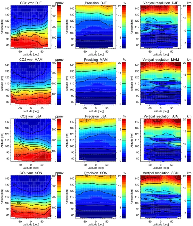
The vertical resolution and the precision are two important parameters for characterizing the quality of any retrieval. The vertical resolution is estimated by the full width at half maximum of the rows of the averaging kernel matrix. Fig-ure 10 shows the zonal means of these parameters calculated from the retrieved data from MIPAS measurements in the UA mode for 2010 and 2011 for each season corresponding to the following months: December–January–February, March– April–May, June–July–August and September–October– November. The zonal mean CO2 distribution is also shown

(left column) for reference.

In general, the precision varies with altitude ranging from

∼1 % below 90 km, 5 % around 120 km and larger than 10 %

above 130 km. The larger values at higher altitudes are due to the lower signal-to-noise ratio. There are some latitudinal and seasonal variations, which are driven mainly by the solar illumination conditions.

The vertical resolution is typically around 5–7 km be-low 120 km. Above that altitude, it is coarser, with values larger than 10 km, mainly caused by the coarser vertical sam-pling (5 instead of 3 km) of the measured spectra. Around

∼105 km, a slight degradation of the vertical resolution is

observed. This altitude corresponds to the tangent height re-gion where the microwindows include lines from the second hot bands only while the fundamental band lines are used above. The latter, as discussed above in Sect. 3, are still rather optically thick at these tangent heights and hence have been rejected.

5.2 Systematic errors

The systematic errors were estimated from the retrieval re-sponse to perturbations in the spectra of the following param-eters: pressure/temperature, O(1_D_{) and O(}3_P_{) abundances,}

MIPAS gain calibration and solar flux. The magnitudes of these perturbations are the same as those used in the retrieval of the collisional rates in Jurado-Navarro et al. (2015) and were already present. There are, however, two exceptions, the temperature, which was assumed with larger errors above 100 km, and the LOS, which was retrieved here and hence its error is already included in the error of the retrieved CO2.

(12)

-50 0 50 Latitude [deg] 80 90 100 110 120 130 140 Altitude [km]

CO2 vmr DJF

50 150 250 350 ppmv 0 100 200 300 400

-50 0 50

Latitude [deg] 80 90 100 110 120 130 140 Altitude [km]

Precision DJF

1 5 15 % 0 5 10 15 20

-50 0 50

Vertical resolution DJF

7 7 15 km 5 10 15 20

-50 0 50

CO2 vmr MAM

50 150 250 350 ppmv 0 100 200 300 400

-50 0 50

Precision MAM

1 5

15 %

0 5 10 15 20

-50 0 50

Vertical resolution MAM

7 7 15 km 5 10 15 20

-50 0 50

CO2 vmr JJA

50 150 250 350 ppmv 0 100 200 300 400

-50 0 50

Precision JJA

1 5 15 % 0 5 10 15 20

-50 0 50

Vertical resolution JJA

7 7 15 km 5 10 15 20

-50 0 50

CO2 vmr SON

50 150 250 350 ppmv 0 100 200 300 400

-50 0 50

Precision SON

1 5 15

15 %

0 5 10 15 20

-50 0 50

Vertical resolution SON

7 7 15 km 5 10 15 20

Figure 10. Latitude-altitude cross sections of CO₂vmr (left column), precision (centre column) and vertical resolution (right column).

The rows, from top to bottom, correspond to the boreal winter (DJF: December–January–February), the vernal equinox (MAM: March– April–May), the austral winter (JJA: June–July–August) and the autumnal equinox (SON: September–October–November). The MIPAS data include the measurements taken in 2010 and 2011 in the UA mode.

95, 100, 110 and≥120 km respectively. Note the change of

sign with altitude introduced by the non-LTE errors. Rezac et al. (2015) used a joint CO2-temperature retrieval

in the analysis of SABER data. Such a retrieval would use a more consistent approach than the joint CO2-LOS retrieval

in the case of MIPAS (below 100 km) since it would

al-low us to diminish the mapping of temperature errors into CO2 errors, though it is more computationally expensive.

We have estimated how much the CO2vmr would be

im-proved in a joint CO2-temperature retrieval, taking the

(13)

of the hydrostatical adjustment of pressure due to the tem-perature changes were taken into account. We only consider the altitudes below 100 km, where the temperature retrieved from the CO215 µm MIPAS spectra is used, and hence the

CO2vmr is needed. In the best case, assuming the CO2vmr

is free of errors in the temperature retrieval, the temperature error would be improved for midlatitude conditions in about 1 K at 85 km and 0.8 K and 0.1 K at 90 and 100 km respec-tively (see Table 2 in García-Comas et al., 2012). For polar summer conditions, the reduction is smaller, 0.7 K at 85 km and 0.1 K at 90–100 km, because non-LTE errors are more relevant. These errors would improve the retrieved CO2

er-ror in 0.7 % at 85 km and only 0.1 % at 90–100 km for the midlatitudes. For polar summer latitudes, the improvements would be even smaller because, at 85 km, the temperature error contribution to the CO2error budget is smaller (see

Ta-ble 1) and, at higher altitudes, because the improvement in the temperature error is not significant. Hence, we expect that the joint CO2-temperature retrieval would not significantly

improve the accuracy of the retrieved CO2vmr.

Regarding the error introduced by the absolute pointing (the error due to the relative pointing, i.e. between adja-cent scans, is already included in the retrieval error since it is jointly retrieved with the CO2vmr), von Clarmann et al.

(2003) estimated the total systematic error in the retrieved ab-solute pointing from 15 µm to be less than 200 m. This error introduces an error in the CO2vmr that is smaller than 1 %

below 90 km, between 1 and 1.5 % at 90–120 km and smaller than 1 % above that altitude. Overall this error is negligible in comparison with the other error sources (see Table 1).

For the atomic oxygen we assumed an uncertainty of 50 %. In view of the recent measurements of O(3_{P )} _by

differ-ent instrumdiffer-ents (see e.g. Kaufmann et al., 2014; Zhu et al., 2015; von Savigny and Lednyts’kyy, 2013; Mlynczak et al., 2013) it might be somehow underestimated. However, un-certainty estimates in this range have been used for the in-version of temperature from SABER measurements (Rems-berg et al., 2008) and from MIPAS spectra (García-Comas et al., 2012, 2014), where the impact of O(3_{P )}_{is larger than}

in the retrieval of CO2; and larger in the retrieval of CO2from

SABER radiances in the same spectral region (4.3 µm) than used here (Rezac et al., 2015). Furthermore, an even smaller error (20 %) has been used in the derivation of thekCO2−O

collisional rate, where the O(3_{P )} _{error has a larger impact}

since it directly propagates into the collisional rate (Feofilov et al., 2012). Thus, in order to make the error budget com-parable with other recent measurements we decided to adopt the same uncertainty of 50 %.

The uncertainty in O(1_D)_{has been considered with}

differ-ent values below about 80 km, where the major production comes from photo-dissociation of O3, and above that

alti-tude, where it is mainly produced by the photo-dissociation of O2. In the stratosphere and lower mesosphere we used the

O3retrieved from simultaneous MIPAS spectra which has an

uncertainty of about 10–15 % (Smith et al., 2013; Glatthor

-20 -10 0 10 20

Retrieval response [%] 60

80 100 120 140

Altitude [km] PT_O(1 D) O(3

P)

Gain

Solar flux

-20 -10 0 10 20

Retrieval response [%] 60

80 100 120 140

Altitude [km] PT_O(1 D) O(3

P)

Gain

Solar flux

(a)

(b)

Figure 11. (a) Systematic errors of the CO₂vmr introduced by

different error sources for midlatitude conditions. CO2 retrieval

responses to individual model parameter perturbations (reflecting their estimated uncertainties) are shown by the coloured lines. The shaded area represents the total systematic error.(b)As(a)but for polar summer conditions.

et al., 2006). Since the photochemical reaction is well known we considered an upper limit error of O3, 15 % for the

O(1D). Above 80 km, the comparison of the photochemical

model of Funke et al. (2012) with the independent model of González-Galindo et al. (2005) give differences smaller than 2 % at all altitudes. Also, the pressure/temperature has been measured with an mean error of about 15 K (see above) and the error of the O2vmr from the NRLMSIS-00 model

is rather small. Therefore, the assumed error of 30 % seems realistic. The other perturbations, which are discussed in de-tail in Jurado-Navarro et al. (2015), are 1.25 % for the gain calibration and 1 % for the solar flux.

In addition, systematic CO2retrieval errors due to

uncer-tainties in the collisional rates used in the non-LTE modelling need to be taken into account. However, since the CO2

colli-sional parameters used here in the CO2inversion have been

retrieved from MIPAS measurement in the same spectral re-gion (see Jurado-Navarro et al., 2015), the CO2retrieval

(14)

er-0 5 10 15 20 25 Total systematic error [%]

60 80 100 120 140

Altitude [km]

Figure 12.Total systematic errors of the main atmospheric

param-eters from the joint CO₂-LOS (black solid line) and CO₂-only (red line) retrievals for midlatitude conditions. The dashed black line shows the total systematic error of the joint CO₂-LOS retrieval for polar summer. The total errors are calculated from the quadratic sum of the retrieval responses to individual model parameter per-turbations shown in Figs. 11a and b.

rors due to collisional rate uncertainties quadratically to the other errors would not be adequate. For instance, it might oc-cur that an overestimation of the solar flux introduces a low bias of a certain collisional rate, but the use of the underesti-mated rate in the CO2retrieval compensates the “direct” CO2

error caused by assuming a solar flux that is too low. There-fore we calculate the1CO2(yi)error due to a given model parameter,yi, i.e. pressure/temperature, O(1D), O(3P), gain calibration and solar flux, by means of

1CO2(yi)= δCO₂

δyi

∀xj=ct e 1yi

+X

j

δCO₂

δxj

1xj(yi),

with1xj(yi)= δx_j

δyi

1yi, (2)

where the second term on the right-hand side accounts for the propagation of the error of model parameters,yi, through the errors in the retrieved collisional parameters, 1xj(yi). The sum extends over the retrieved collisional parameters, xj:

kvv2,kvv3,kvv4,kF1,kF2andfvt, which have errors due to the model parametersyi,1xj(yi)listed in Table 3 of Jurado-Navarro et al. (2015). The first term on the right-hand side, where1yi is the error of model parameteryi, has been dis-cussed above. The total systematic error in CO2is then

calcu-lated by a quadratic sum over the errors of all model parame-ters,1COTotal₂ =

q P

i[1CO2(yi)]2. The resulting corrected retrieval responses to the model parameter perturbations (re-flecting their estimated uncertainties) are shown in Fig. 11a and b and are listed in Table 1 for some altitudes.

The calculations indicate that the largest error contribution above 100 km comes from the pressure/temperature uncer-tainties for both considered atmospheric conditions, reaching values up to∼15–16 % in midlatitude conditions (Fig. 11a)

and ∼20 % in polar summer conditions (Fig. 11b).

Be-low, the pressure/temperature error maximizes again around 80 km, with maximum values at midlatitude conditions of up to∼4 %. The MIPAS gain calibration and solar flux

uncer-tainties introduce errors of 2–3 % from 85 up to 110 km in both conditions. The total error below 90 km in polar sum-mer conditions is indeed dominated by these uncertainties. The O(1D)and O(3P ) uncertainties have a non-negligible

contribution above 95 km with the largest values up to 4 % at 105 km in polar summer conditions.

It is important to highlight that, in polar summer condi-tions, the MIPAS temperature retrieved from the NO 5.3 µm emission is smaller than MSIS (Mass Spectrometer and Inco-herent Scatter) temperatures in up to 10 K in the lower ther-mosphere (Bermejo-Pantaleón et al., 2011). Thus, the use of thermospheric MIPAS temperature, instead of MSIS, in-creases the retrieved CO2vmr by up to 15 % under these

par-ticular conditions.

Regarding the effects of the joint CO2-LOS retrieval on

the total systematic error, Fig. 12 shows that it is notably larger for the CO2-only retrieval than for the joint CO2-LOS

retrieval. This indicates that a large fraction of the spectral residuals due to the systematic errors of the different param-eters is compensated by the LOS in the joint retrieval while in the CO2-only retrieval all errors map onto the CO2vmr

pro-file. In this sense, the joint CO2-LOS retrieval is also useful

for dampening systematic errors of the retrieved CO2vmr.

Deviations of the retrieved profile from the true profile when perturbing the a priori profile are often called smooth-ing errors. However, while it is important to assess the sen-sitivity of the retrieval to the a priori profile shape as we do above, we do not include smoothing errors in the over-all error budget. Firstly, because the concept of “smoothing errors” itself is questionable (von Clarmann, 2014) and, sec-ondly, because these deviations can be implicitly accounted for in comparisons to model simulations or independent ob-servations by applying the MIPAS averaging kernels to the latter.

One important result that should be mentioned is that the systematic errors obtained here in the retrieved CO2vmr are

much smaller than those obtained before in previous mea-surements of CO2using limb emission measurements of the

4.3 µm atmospheric radiance (e.g. López-Puertas et al., 1998; Kaufmann et al., 2002; Rezac et al., 2015). The main reasons are as follows. Firstly, more accurate non-LTE collisional rates have been used, enabled by the high-resolution MIPAS spectra (see Jurado-Navarro et al., 2015). Secondly, the wide spectral range, together with the high spectral resolution of MIPAS, has allowed the retrieval of the temperature and O3

up to about 100 km, and the temperature in the lower ther-mosphere (up to∼170 km) before the CO₂vmr. The use of

these concentrations has significantly reduced the systematic error of CO2.

(15)

Apr 2010

0 100 200 300 400 500

CO2 volume mixing ratio (ppmv) 60

80 100 120 140

Altitude

(

km

)

Dec 2010

0 100 200 300 400 500

CO2 volume mixing ratio (ppmv) 60

80 100 120 140

Altitude (km)

Figure 13.Examples of the CO2vmr profiles measured by MIPAS during 2010 for April (equinox, left) and December (solstice, right).

the auroral region is the excitation of CO2(v3) viaV−V

en-ergy transfer from N2(v) which is excited by auroral

elec-trons. However, its importance during daytime conditions seems to be negligible, much smaller than the solar absorp-tion at 4.3 and 2.7 µm since SABER CO24.3 µm radiance

measurements show that the daytime signal is more than 2 orders of magnitude larger than the night-time signal in the auroral regions.

The possible excitation of CO2by “hot” O atoms was

pos-tulated by Feofilov et al. (2012) as an additional source of the excitation of CO2(v2) (15 µm) in order to understand the

differences between the collisional rates of CO2-O measured

in the laboratory and those derived from atmospheric mea-surements. Sharma (2015) found, however, that the chance of a hot atom colliding with CO2is virtually nil in the

meso-sphere and lower thermomeso-sphere. The excitation of CO2in the

more energetic v3 state would then be even less probable.

Thus, as there is no evidence of such excitation mechanism for CO2(v3), its inclusion is not justified. We should also note

that this mechanism was not included in the recent retrieval of CO2from SABER measurements (Rezac et al., 2015).

In this work we have not included rotational non-LTE. Based on previous assessments (Gusev, 2002), rotational non-LTE in the CO2(v3) ro-vibrational states (emitting in the

fundamental band used here in the retrieval of CO2 above

100 km, where rotational non-LTE has a larger propensity to occur) is likely to introduce only marginal errors in the verti-cal range of interest (70–140 km), being negligible compared to other error sources.

6 MIPAS CO2climatology for 2010–2011

Figure 14a and b shows the monthly zonal mean CO2vmr

retrieved from MIPAS daytime spectra taken in its upper at-mosphere (UA) mode. The figure shows the major features expected for the CO2distribution and predicted by models.

Compare, for example, the CO2zonal mean distributions

ob-tained by the CMAM model for April and August (middle panel of the upper row in Fig. 3 and top-right panel in Fig. 8 in Beagley et al., 2010), with the corresponding months in Fig. 14a and b. Also the similar broad features are shown by the WACCM-SD model simulations (see the upper pan-els of Fig. 3 in Garcia et al., 2014 for February and April). Those features comprise the abrupt decline of the CO2vmr

above around 80–90 km. The other major feature is the sea-sonal change of the latitudinal distribution, leading to higher CO2vmr from 70 up to ∼95 km in the polar summer,

in-duced by the ascending branch of the mean circulation, and lower CO2abundances, with respect to the tropics and polar

summer, at the same altitudes in the polar winter region. It is noticeable that the distribution reverses above∼95 km, CO₂

being more abundant in the polar winter region than at the midlatitudes and polar summer; also as a consequence of the reversal of the mean circulation (see e.g. Smith et al., 2011). The solstice seasonal distribution, with a significant pole-to-pole CO2gradient lasts about 2.5 months in each hemisphere

(November to February and May to August), while the sea-sonal transition occurs quickly, mainly in April and October. Another observed feature is the rapid increase of CO2vmr

from mid-high latitudes towards the polar regions in the lower thermosphere during the equinoxes (more evident in April and October). We cannot find any physical reason for it and we do not discard that this could be a retrieval artefact caused by the inversion of CO2 in conditions of very high

(>80◦) solar zenith angles.

A comparison of the MIPAS CO2vmr with ACE

(16)

MIPAS v622. Jan 2010-2011

-90 -60 -30 0 30 60 90

Latitude (deg) 60 80 100 120 140 Altitude (km) 50 50 75 100 150 200 250 300 350 375 (ppmv) 100 200 300 400

MIPAS v622. Feb 2010-2011

-90 -60 -30 0 30 60 90

Latitude (deg) 60 80 100 120 140 Altitude (km) 25 50 50 75 75 100 150 200 250 250 300 300 350 375 375 (ppmv) 100 200 300 400

MIPAS v622. Mar 2010-2011

-90 -60 -30 0 30 60 90

Latitude (deg) 60 80 100 120 140 Altitude (km) 25 50 50 75 75 100 150 200 250 300 300 350 350 375 375 (ppmv) 100 200 300 400

MIPAS v622. Apr 2010-2011

-90 -60 -30 0 30 60 90

Latitude (deg) 60 80 100 120 140 Altitude (km) 25 50 50 75 75 100 100 150 150 200 250 250 300 350 375 375 (ppmv) 100 200 300 400

MIPAS v622. May 2010-2011

-90 -60 -30 0 30 60 90

Latitude (deg) 60 80 100 120 140 Altitude (km) 25 50 50 75 75 100 150 200 250 300 350 375 375 (ppmv) 100 200 300 400

MIPAS v622. Jun 2010-2011

-90 -60 -30 0 30 60 90

Latitude (deg) 60 80 100 120 140 Altitude (km) 25 50 50 75 100 150 200 250 300 350 375 375 (ppmv) 100 200 300 400 (a) Figure 14. 7 Conclusions

We have retrieved global distributions of the CO2vmr

(vol-ume mixing ratio) in the mesosphere and thermosphere (from 70 up to∼140 km) for MIPAS daytime high-resolution

spec-tra. This is the first time that the relative CO2concentration

(vmr, not the CO2number density) has been retrieved in the

mid-thermosphere (120–140 km). The retrieved CO2has an

improved accuracy because of the new rate coefficients re-cently derived from MIPAS (Jurado-Navarro et al., 2015),

and the simultaneous MIPAS measurements of other key at-mospheric parameters (retrieved in previous steps) needed for the non-LTE modelling like the temperature in the meso-sphere and in the thermomeso-sphere, as well as the O3

(17)

MIPAS v622. Jul 2010-2011

-90 -60 -30 0 30 60 90

Latitude (deg) 60 80 100 120 140 Altitude (km) 50 50 75 100 150 200 250 300 350 375 375 (ppmv) 100 200 300 400

MIPAS v622. Aug 2010-2011

-90 -60 -30 0 30 60 90

Latitude (deg) 60 80 100 120 140 Altitude (km) 25 50 50 75 ₇₅ 100 150 200 250 300 350 375 (ppmv) 100 200 300 400

MIPAS v622. Sep 2010-2011

-90 -60 -30 0 30 60 90

Latitude (deg) 60 80 100 120 140 Altitude (km) 25 50 50 75 75 100 100 150 150 200 250 250 300 350 350 375 375 (ppmv) 100 200 300 400

MIPAS v622. Oct 2010-2011

-90 -60 -30 0 30 60 90

Latitude (deg) 60 80 100 120 140 Altitude (km) 25 50 50 75 75 100 150 150 200 200 250 250 300 300 350 350 375 375 (ppmv) 100 200 300 400

MIPAS v622. Nov 2010-2011

-90 -60 -30 0 30 60 90

Latitude (deg) 60 80 100 120 140 Altitude (km) 25 50 75 100 150 200 250 300 350 375 (ppmv) 100 200 300 400

MIPAS v622. Dec 2010-2011

-90 -60 -30 0 30 60 90

Latitude (deg) 60 80 100 120 140 Altitude (km) 25 25 50 75 100 150 200 250 300 350 375 (ppmv) 100 200 300 400 (b)

Figure 14. (a)Monthly zonal mean CO₂vmr measured by MIPAS during the 2010–2011 period for the UA mode for months of January to

June.(b)As(a)but for months of July to December.

The CO2vmrs have been retrieved using MIPAS daytime

limb emission spectra from the 4.3 µm region in its upper atmosphere (UA) mode (data version v5r_CO2_622). Night-time spectra were not used because they are very noisy and the non-LTE processes operating at night are not known very accurately. The retrieved CO2covers from 70 km up to about

140 km and all latitudes except in the dark regions of the po-lar winter. The inversion of CO2has been performed jointly

with the line of sight (LOS) by using a non-LTE retrieval

scheme developed at IAA/IMK. It takes advantage of other (simultaneous) MIPAS measurements of atmospheric param-eters (retrieved in previous steps), such as the kinetic tem-perature (up to∼100 km) from the CO₂15 µm region, the

thermospheric temperature from the NO 5.3 µm, the O3

mea-surements (up to∼100 km), which allows a strong constraint

on the O(1_D_{) concentration below}_∼_{100 km, and an accurate}

calculation of O(1_D_{) above}_∼_{100 km. The non-LTE model}

(18)

vibrational–translational collisional rates retrieved from the MIPAS spectra.

The precision of the retrieved CO2vmr profiles varies with

altitude, ranging from ∼1 % below 90 km to 5 % around

120 km and larger than 10 % above 130 km. The larger values at higher altitudes are due to the lower signal-to-noise ratio. There are very few latitudinal and seasonal variations of the precision, which are mainly driven by the solar illumination conditions. The retrieved CO2profiles have a vertical

reso-lution of about 5–7 below 120 km and between 10 and 20 at 120–140 km.

Retrieval simulations performed with synthetic spectra have demonstrated that the developed CO2-LOS joint

re-trieval allows for a rere-trieval of the CO2 profile in the 70–

140 km range with high accuracy. The use of strongly per-turbed a priori CO2 and LOS information results in very

small different between the true and the retrieved profiles, generally smaller than 2–3 % in the midlatitudes and smaller than 2 % (except near 95–110 km where it ranges at 2–4 %) for polar summer conditions. We have also proven that the algorithm is capable of retrieving unusual CO2profiles such

as those showing a low vmr between 70 and 85 km and a pro-nounced peak near 90 km, and also CO2profiles affected by

wave propagation. The retrieval scheme clearly discriminates the information of CO2 concentration from the LOS. The

mapping of typical CO2 a priori uncertainties on the LOS

is very small (less than 20 m), and a deviation in the a pri-ori LOS profile of 200 m introduces a change in the retrieved CO2profile smaller than 1–2 %. We have also found that the

systematic errors are significantly reduced when using the CO2-LOS joint retrieval instead of the CO2-only scheme.

The major systematic error source is the uncertainty of the pressure/temperature profiles, retrieved also from MI-PAS spectra, near 15 µm below 100 km (García-Comas et al., 2014) and from 5.3 µm above 100 km Bermejo-Pantaleón et al. (2011). They can induce a systematic error at midlat-itude conditions of up to 15 % above 100 km (20 % for polar summer conditions) and of ∼5 % around 80 km. The

sys-tematic errors due to uncertainties of the O(1_D_{) and O(}3_P₎

profiles are within 3–4 % in the 100–120 km region. The er-rors due to uncertainties in the gain calibration and in the solar flux at 4.3 and 2.7 µm are within∼2 % at all altitudes.

The most important features observed on the retrieved CO2can be summarized as follows:

– The retrieved CO2 shows the major general features

expected and predicted by models: the abrupt decline of the CO2vmr above 80–90 km, caused by the

pre-dominance of the molecular diffusion and the seasonal change of the latitudinal distribution. The latter is re-flected by higher CO2 abundances in polar summer

from 70 km up to ∼95 km and lower CO₂vmr in the

polar winter, both induced by the ascending and de-scending branches of the mean circulation respectively. Above∼95 km, CO₂is more abundant in the polar

win-ter than at the midlatitudes and polar summer regions, caused by the reversal of the mean circulation in that altitude region.

– The solstice seasonal distribution, with a significant pole-to-pole CO2 gradient lasts about 2.5 months in

each hemisphere (November to February and May to August), while the seasonal transition occurs quickly, mainly in April and October.

8 Data availability

The retrieved CO2 volume mixing ratio data version

v5r_CO2_622 will be made available at the IMK-IAA MI-PAS data set website: https://www.imk-asf.kit.edu/english/ 308.php, once the final processing is finished.

The Supplement related to this article is available online at doi:10.5194/amt-9-6081-2016-supplement.

Acknowledgements. The IAA team was supported by the Spanish

MCINN under grant ESP2014-54362-P and EC FEDER funds. Maya García-Comas was financially supported by the Ministry of Economy and Competitiveness (MINECO) through its “Ramón y Cajal” subprogramme. The authors acknowledge ESA for providing MIPAS L1b spectra.

Edited by: S. Kirkwood

Reviewed by: A. Feofilov and one anonymous referee

References

Beagley, S. R., Boone, C. D., Fomichev, V. I., Jin, J. J., Semeniuk, K., McConnell, J. C., and Bernath, P. F.: First multi-year occul-tation observations of CO₂in the MLT by ACE satellite: obser-vations and analysis using the extended CMAM, Atmos. Chem. Phys., 10, 1133–1153, doi:10.5194/acp-10-1133-2010, 2010. Bermejo-Pantaleón, D., Funke, B., Lopez-Puertas, M.,

García-Comas, M., Stiller, G. P., von Clarmann, T., Linden, A., Grabowski, U., Höpfner, M., Kiefer, M., Glatthor, N., Kellmann, S., and Lu, G.: Global Observations of Thermospheric Tempera-ture and Nitric Oxide from MIPAS spectra at 5.3 µm, J. Geophys. Res., 116, A10313, doi:10.1029/2011JA016752, 2011.

De Laurentis, M.: Planning of MIPAS new special modes January 2005 Campaign, Tech. rep., ESA Technical Note, ENVI-SPPA-EOPG-TN-05-0002, 2005.