Estimating the flood frequency distribution at seasonal and annual time scale

(1)

HESSD

9, 7947–7967, 2012

Seasonal flood frequency analysis

E. Baratti et al.

Title Page

Abstract Introduction

Conclusions References

Tables Figures

◭ ◮

Back Close

Full Screen / Esc

Printer-friendly Version Interactive Discussion

Discussion

P

a

per

|

Dis

cussion

P

a

per

|

Discussion

P

a

per

|

Discussio

n

P

a

per

|

Hydrol. Earth Syst. Sci. Discuss., 9, 7947–7967, 2012 www.hydrol-earth-syst-sci-discuss.net/9/7947/2012/ doi:10.5194/hessd-9-7947-2012

Hydrology and Earth System Sciences Discussions

This discussion paper is/has been under review for the journal Hydrology and Earth System Sciences (HESS). Please refer to the corresponding final paper in HESS if available.

Estimating the flood frequency

distribution at seasonal and

annual time scale

E. Baratti1, A. Montanari1, A. Castellarin1, J. L. Salinas2, A. Viglione2, and A. Bezzi3

1

School of Civil Engineering (Dept. DICAM), University of Bologna, Italy

2

Institute of Hydraulic Engineering and Water Resources Management, Vienna University of Technology, Austria

3

Studio Ing. G. Pietrangeli S.r.l. – Via Cicerone 28 Rome, Italy

Received: 31 May 2012 – Accepted: 8 June 2012 – Published: 27 June 2012 Correspondence to: E. Baratti ([email protected])

(2)

HESSD

9, 7947–7967, 2012

E. Baratti et al.

Title Page

Tables Figures

◭ ◮

Back Close

Full Screen / Esc

Discussion

P

a

per

|

Dis

cussion

P

a

per

|

Discussion

P

a

per

|

Discussio

n

P

a

per

|

Abstract

We propose an original approach to infer the flood frequency distribution at seasonal and annual time scale. Our purpose is to estimate the peak flow that is expected for an assigned return periodT, independently of the season in which it occurs (i.e. annual flood frequency regime), as well as in different selected sub-yearly periods (i.e.

sea-5

sonal flood frequency regime). While a huge literature exists on annual flood frequency analysis, few studies have focused on the estimation of seasonal flood frequencies despite the relevance of the issue, for instance when scheduling along the months of the year the construction phases of river engineering works directly interacting with the active river bed, like for instance dams. An approximate method for joint frequency

10

analysis is presented here that guarantees consistency between fitted annual and sea-sonal distributions, i.e. the annual cumulative distribution is the product of the seasea-sonal cumulative distribution functions, under the assumption of independence among floods in di_fferent seasons. In our method the parameters of the seasonal frequency distribu-tions are fitted by maximising an objective function that accounts for the likelihoods of

15

both seasonal and annual peaks. Differently from previous studies, our procedure is conceived to allow the users to introduce subjective weights to the components of the objective function in order to emphasize the fitting of specific seasons or of the annual peak flow distribution. An application to the time series of the Blue Nile daily flows at Sudan-Ethiopia border is presented.

20

1 Introduction

Flood frequency analysis is often used by practitioners to support the design of river en-gineering works, flood mitigation procedures and civil protection strategies. It is gener-ally carried out by fitting peak flow observations by using a suitable probability distribu-tion. Two approaches are mainly applied. Using an annual maximum series (AM), one

25

(3)

HESSD

9, 7947–7967, 2012

E. Baratti et al.

Title Page

Tables Figures

◭ ◮

Back Close

Full Screen / Esc

Discussion

P

a

per

|

Dis

cussion

P

a

per

|

Discussion

P

a

per

|

Discussio

n

P

a

per

|

or peak-over-threshold method (POT), the analysis considers all peaks above a given threshold level (e.g. Madsen et al., 1997a,b).

In many practical cases one is also interested in inferring the flood frequency distri-bution for given intra–annual periods, for instance when one needs to estimate the risk of flood in different seasons. Such information is needed when planning the

construc-5

tion phases of river engineering works whose building area is in close proximity to the active river bed for various months or years.

There are several problems encountered when fitting seasonal and annual frequency curves independently and a key issue is to ensure the compatibility between intra– annual and annual flood probability distributions. One example is the problem of

cross-10

ing over: in the probability plot, the annual distribution must always lie on or above the highest seasonal distribution (Durrans et al., 2003), i.e. the probability of one peak value of being exceeded in the entire year must be higher than the probability of the same value of being exceeded in one season. The issue of seasonal flood frequency analysis was considered by Creager et al. already in 1951. However, literature

ded-15

icated little attention to this problem in comparison with the estimation of annual ex-tremes. In fact, several contributions dealt with intra-annual flood assessment but in many cases the purpose was to support with seasonal information the estimation of the annual peak flow. For instance, Stedinger et al. (1992) discussed the advantages and drawbacks related to using seasonal flow data to estimate the annual peak flow

dis-20

tribution but did not explicitly focus on flood estimation in sub-yearly periods. Similarly, Kochanek et al. (2012) and Strupczewski et al. (2012) focused on the upper quantiles of the annual peak flows by fitting data collected in two seasons. Other analogous con-tributions were provided by Buishand and Demar `e (1990), who refer to rainfall depths, and Singh et al. (2005). Among the contributions that are explicitly dedicated to

infer-25

(4)

HESSD

9, 7947–7967, 2012

E. Baratti et al.

Title Page

Tables Figures

◭ ◮

Back Close

Full Screen / Esc

Discussion

P

a

per

|

Dis

cussion

P

a

per

|

Discussion

P

a

per

|

Discussio

n

P

a

per

|

on adapting the skewness coefficient of seasonal distributions to ensure a satisfactory fit of the annual peak flows, thereby putting more emphasis on the annual distribution. Allamano et al. (2011) analyze the magnitude of under- (or over-) estimation of design events in the presence of seasonality by using the POT or AM approach. Bowers et al. (2012) presents a statistical procedure to partition river flow data into three seasons

5

and focuses on two particular distributions to describe the constructed seasonal river flows: power law and lognormal. Fang et al. (2007) proposed an approach based on the peaks-over-threshold sampling method and a non-identical Poisson distribution to model the flood occurrence within each season. Another relevant contribution was re-cently given by Chen et al. (2010) who proposed the use of a copula function to jointly

10

model the distributions of flood magnitude and date of occurrence. We propose a prac-tical and useful alternative approach for jointly estimating seasonal and annual flood frequency distributions, which has the relevant feature that, under the assumption of mutual independence of seasonal peaks, the number of seasons and their distribution along the year can be defined with great flexibility. In detail, we analyse yearly

max-15

ima collected at seasonal and annual time scale and develop an objective function for parameter estimation, which consists in the weighted sum of seasonal and annual log-likelihoods for the peaks of being observed. Parameters of the seasonal distributions are optimised while, under the assumption of independence of the flood generating process among seasons, the annual distribution is computed as the product of the

20

seasonal ones. Likelihood weights can be used to put more emphasis on one or more distributions, whether sub-yearly or annual. It is worth noting that the optimisation pro-cedure is similar to a maximum likelihood estimation, but our objective function is not a likelihood function since combines seasonal and annual likelihoods and allow the user to assign weights to them. The method represents an approximate solution to

25

(5)

HESSD

9, 7947–7967, 2012

E. Baratti et al.

Title Page

Tables Figures

◭ ◮

Back Close

Full Screen / Esc

Discussion

P

a

per

|

Dis

cussion

P

a

per

|

Discussion

P

a

per

|

Discussio

n

P

a

per

|

With respect to the approach proposed by Chen et al. (2010) our method ensures more flexibility in the choice of the seasons which can eventually be very different in terms of their impact on the annual flood distribution. For illustration purposes, the proposed approach is applied to infer seasonal and annual flood frequency distributions for the Nile River at the Sudan-Ethiopia border.

5

2 Parameterisation of seasonal and annual flood frequency distributions

Let us define a season as a contiguous period of the year with its own river flow regime and seasonal flood frequency distribution. Assuming that the year is divided into N

seasons in which flood distributions are independent of each other, the cumulative probability distribution function (CDF) of the annual maximum flood F_Q

Y is given by 10

(e.g. Waylen and Woo, 1982; Durrans et al., 2003)

F_Q Y(q|(

θ₁_,_{. . .}_,θ_N₎₎₌

N

Y

i₌1

F_Q

i(q|θi), i =1,. . .,N (1)

whereF_Q

i and θi are the CDF and the vector of the parameters for seasoni,

respec-tively. This relationship clearly shows that seasonal and annual probability distributions are strictly related, meaning that the estimation of their parameters should be

condi-15

tioned by Eq. (1). The literature has proposed several methods to impose the afore-mentioned condition. For instance, Durrans et al. (2003) conditioned the skewness coe_fficients of seasonal distributions to fit the annual flood frequency behaviors.

One should note that the dependency among seasonal and annual peak flow dis-tributions implies that the yearly peak flow estimated by seasonal maxima discharge

20

(6)

HESSD

9, 7947–7967, 2012

E. Baratti et al.

Title Page

Tables Figures

◭ ◮

Back Close

Full Screen / Esc

Discussion

P

a

per

|

Dis

cussion

P

a

per

|

Discussion

P

a

per

|

Discussio

n

P

a

per

|

Under the assumption of independence among seasonal peak flows, we propose an estimation technique for seasonal and annual flood frequency distributions which enables the user to (a) select the seasons independently of their significance in the for-mation of the overall flood regime, (b) assign different weights to the fitting of seasonal and annual distributions and (c) overcome the problem of the crossing over among

5

seasonals and annual distributions.

The method makes use of the annual maxima sampling method to select relevant floods at seasonal and annual time scale and is articulated in the following steps.

1. From the observed data series, select the sample of the annual maximum peak flows (AM), as well as the samples collecting the annual maxima in each season

10

(SMi).

2. For the above seasonal samples, identify a suitable probability distribution and es-timate its parameters, for instance by using the L-moments method (e.g. Hosking and Wallis, 1997) (i.e. initial parameter set).

3. Compute the objective functionξ(θ₁_,_{. . .}_,θ_N_{) for the joint-estimation of seasonal} 15

and annual distributions parameters through the relationship

ξ(θ₁_,_{. . .}_,θ_N₎₌

N

X

i=1

 

 w_i

M_Si

X

j=1

lnhf_Q

i(qSi,j|θi) i

 

 +w_Y

MY X

k=1

lnhf_Q

Y(qY,k|(θ1,. . .,θN)) i

(2)

whereM_S

i andMY are the samples sizes of SMi and AM, respectively, which may

be different (e.g. the case of seasons affected by missing data);q_S

i,j andqY,k are

the observations in SMi and AM, respectively;fQi(qSi,j|θi) andfQY(qY,k|θ1, ...θN) 20

are the seasonal and annual probability density functions;w_i and w_Y, with w_Y ₊ PN

(7)

HESSD

9, 7947–7967, 2012

E. Baratti et al.

Title Page

Tables Figures

◭ ◮

Back Close

Full Screen / Esc

Discussion

P

a

per

|

Dis

cussion

P

a

per

|

Discussion

P

a

per

|

Discussio

n

P

a

per

|

distributions given the observed intra–annual and annual peak discharges. In view of Eq. (1), the annual log-likelihood, presents in the second term at the right hand side of Eq. (2), can be computed by

lnhf_Q

Y(qY,k|(θ1,. . .,θN)) i

=ln

" _N X

i=1

f_Q

i(qY,k|θi)

N

Y

j=1 j6=i

F_Q

J(qY,k|θj) !#

. (3)

Since Eq. (2) depends only by seasonal parametersθ

1,. . .,θN.

5

4. Through an optimization algorithm maximize the objective function given by Eq. (2) therefore identifying the best parameter set (i.e. optimal parameter set).

Weights in Eq. (2) are introduced to control the relevance of the fit of each single frequency distribution in the overall procedure. Weights are necessary because Eq. (2) is a fit-for-purpose procedure that makes a redundant use of the annual maximum peak

10

flow, whose frequency distribution is used twice to assign a priority, if needed, to the fit of the annual distribution with respect to the related seasonal ones. With a proper choice of weights, the proposed procedure may converge to the traditional procedure that is based on the analysis of annual maxima only. One application of the proposed approach is presented in the following section.

15

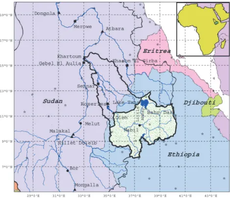
3 Application to the Blue Nile River at Sudan-Ethiopia Border

The proposed method was used to estimate the flood frequency distribution, by refer-ring to di_fferent yearly subperiods, for the Blue Nile River at Sudan-Ethiopia Border. The Blue Nile originates from Lake Tana, in Ethiopia. Together with the White Nile, it is one of the major tributaries of the Nile River. The main stream length at Sudan

Bor-20

(8)

HESSD

9, 7947–7967, 2012

E. Baratti et al.

Title Page

Tables Figures

◭ ◮

Back Close

Full Screen / Esc

Discussion

P

a

per

|

Dis

cussion

P

a

per

|

Discussion

P

a

per

|

Discussio

n

P

a

per

|

the Blue Nile contribution. Figure 1 shows a schematic representation of the Blue Nile watershed.

Daily river flow observations that were collected by the Ethiopian Ministry of Irrigation and Water Resources (MoWR) between 1961 and 2005 (i.e. 45 yr) are available at Su-dan Border. Nevertheless, the series is a_ffected by several missing data, mainly from

5

January to June/July, therefore the number of usable years is less than 45. In particular, we retained in the annual maximum series of flood flows only the 25 yr for which daily observations are available during the whole wet season (i.e. from June to September, see Rientjes et al., 2011). Concerning seasonal sub-samples, we included the sea-sonal maximum daily discharge in the seasea-sonal database only when observations are

10

available for at least 70 % of thei-th season.

The maximum annual flood of the Blue Nile exhibits a very strong seasonality and is characterized by one peak season, as it is common in monsoon–dominated cli-mates. Indications reported in the literature (e.g. Rientjes et al., 2011) distinguishes two main climatic seasons for the study area, namely: a wet (i.e. from June to

Septem-15

ber) and a dry (i.e. from October to May) season, while in the easternmost part of the study area a subdivision into three climatic seasons is suggested by some au-thors (e.g. Seleshi and Camberlin, 2006): Kiremt (“main rains”, heavy rainy season, June–September), Belg (“small rains”, light rainy season, February–May), and the dry season Bega (October–January). During the wet season the contribution of the Blue

20

Nile is about two thirds of the flow of the receiving Nile.

3.1 Season identification

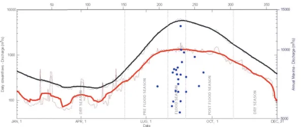
In order to identify the optimal number of seasons, climatic behaviours were considered along with the practical need to estimate peak flows in assigned periods for water resources management purposes. To obtain a first picture of climatic behaviours, Fig. 2

25

(9)

HESSD

9, 7947–7967, 2012

E. Baratti et al.

Title Page

Tables Figures

◭ ◮

Back Close

Full Screen / Esc

Discussion

P

a

per

|

Dis

cussion

P

a

per

|

Discussion

P

a

per

|

Discussio

n

P

a

per

|

(red thick line), while annual maximum peak flows are indicated as blue dots. It can be seen that seasonality is very pronounced with one flood season only.

Directional statistics were used to quantify seasonality of flood events (Mardia, 1972) on the basis of the timing of annual maximum flood flows. After Bayliss and Jones (1993), the date of occurrence of the eventi can be written as a directional statistic by

5

converting the Julian date, Jd, of occurrence into an angular measure given by

ϕ_i ₌Jd_i

2π

365

. (4)

Therefore, each date of occurrence can be represented in polar coordinates as a vector with a unit magnitude and a direction given by Eq. (4). This allows the determination of thexandy coordinates of the mean of a sample ofZ dates of occurrence as

10

x₌ 1 Z

Z

X

i=1

cos(ϕ_i);y ₌ 1 Z

Z

X

i=1

sin(ϕ_i) . (5)

Therefore, the directionϕ, along with the magnitude,r, of the vector representing this point in polar coordinates, can be obtained by

ϕ₌arctany

x

, (6)

r₌ q

x2₊_y2_. ₍₇₎

15

Equation (6) represents a measure of the mean timing for the sample ofZ dates, such as the days of occurrence in an annual maximum series, and can be converted back to a mean date, MD, through

MD=ϕ

365 2ϕ

. (8)

(10)

HESSD

9, 7947–7967, 2012

E. Baratti et al.

Title Page

Tables Figures

◭ ◮

Back Close

Full Screen / Esc

Discussion

P

a

per

|

Dis

cussion

P

a

per

|

Discussion

P

a

per

|

Discussio

n

P

a

per

|

Equation (7) gives a measure of the regularity of the phenomenon: values ofr close to one imply a strong seasonality, or regularity, in the dates of occurrence of the events, values close to zero are symptomatic of a great dispersion throughout the year.

Through directional statistics the limits of the flood season,ϕ₁andϕ₂, are quantita-tively identified through the relationship

5

ϕ_1,2₌ϕ±σ, (9)

where the negative and positive signs correspond to the beginning and the end of the season, respectively, andσis the standard deviation in radiants given byσ₌p−2 ln (r) (Mardia, 1972). The computed mean angular measures are converted back to calendar dates by using Eq. (8).

10

Directional statistics were applied to annual maximum series (AM) of daily stream-flows of the Blue Nile at Sudan-Ethiopia Border. The results show that the annual max-imum flood is extremely regular, with measure of regularity equal to r₌0.977 (it is relevant to note that r₌1 would correspond to observed annual maxima happening on the same day of the year). Most of the observed flood dates falls within the 3-week

15

time period from 31 July to 25 August. We identify this period as the flood season. Fur-thermore, we identify three additional seasons to fully characterize the high streamflow regime (see Fig. 2), by also taking practical need of water resources management into account: a dry season from 1 November to 31 May; a pre-flood season from 1 June to 30 July, and a post flood season from 26 August to 31 October. For each of the

20

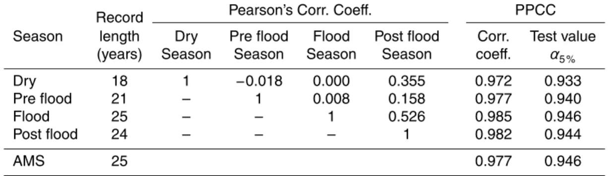
above periods, the seasonal maximum daily discharge was extracted. Table 1 presents the record length in years of each seasonal sample as well as the unique sample composed by the annual peak discharge. The matrix of the Pearson’s correlation coef-ficients between the different samples is also shown in Table 1.

It can be seen that the null hypothesis of statistical mutual independence of seasonal

25

(11)

HESSD

9, 7947–7967, 2012

E. Baratti et al.

Title Page

Tables Figures

◭ ◮

Back Close

Full Screen / Esc

Discussion

P

a

per

|

Dis

cussion

P

a

per

|

Discussion

P

a

per

|

Discussio

n

P

a

per

|

It is relevant to point out that, in principle, the number of seasons and their calendar limits can be defined arbitrarily. However, for increasing number of seasons one expe-riences a higher chance of detecting correlation among them. It is also significant to note that season identification based on climatic behaviours, rather than an arbitrary selection, leads to yearly subperiods that are well distinguished from a climatic point

5

of view and therefore are more likely to be independent (e.g. Waylen and Woo, 1982; Durrans et al., 2003; Strupczewski et al., 2012; Kochanek et al., 2012).

3.2 Estimation of seasonal and annual flood frequency distributions

Table 1 reports the results of the Plotting Position Correlation-Coe_fficient (PPCC) test (e.g. Vogel, 1986; Castellarin et al., 2004) that was carried out to test the

suitabil-10

ity of the Gumbel distribution (also called EV1 distribution) to simulate the flood fre-quency behaviours in each season. For all seasons the linear correlation coe_fficient is reported between seasonal flood flows and their sample non-exceedance proba-bility expressed through the Gumbel reduced variate (i.e. y₌−ln (−ln (F)), where F

indicates the nonexceedance probability). The test value for a 5 % significance level is

15

also given. It can be seen that the Gumbel distribution can never be rejected at the 5 % significance level for all the seasons. Therefore, initial values for the distribution param-eters were estimated through the L-moments method (Hosking and Wallis, 1997) (see Table 2).

Through a genetic algorithm (Mebane and Sekhon, 2011), the seasonal

distribu-20

tion parameters were obtained by maximizing Eq. (2). Figure 3 shows in a Gumbel probability plot the initially fitted seasonal distributions (dotted lines) along with the sample frequency of the observed data (dots) and the final seasonal distributions re-sulting from the proposed approach (continuous lines) by adopting uniform weights. The annual CDF obtained from individual fitting of annual maxima and joint estimation

25

(12)

HESSD

9, 7947–7967, 2012

E. Baratti et al.

Title Page

Tables Figures

◭ ◮

Back Close

Full Screen / Esc

Discussion

P

a

per

|

Dis

cussion

P

a

per

|

Discussion

P

a

per

|

Discussio

n

P

a

per

|

cross the independently fitted annual distribution (blue dashed-dotted line). The sea-sonal distribution parameters, given by initial fitting and jointly fitting, are summarised in Table 2.

Figure 3 shows a fair-to-good agreement between sample, individually fitted and joint estimated distributions, although some slight discrepancy is detected, as expected.

5

In particular, the individually (independently) fitted seasonal distributions are overesti-mated while the contrary holds for the individually fitted annual distribution.

It can be also seen that the e_ffect of dependence on the fitting of the post flood and the flood season, namely, the difference between independent and joint estimates, is indeed negligible. As it was expected for the given climate, it can be seen that the

10

annual distribution is similar to that of the dominant flood season (Strupczewski et al., 2012; Kochanek et al., 2012).

In Fig. 4 the sensitivity of the method to the choice of weights is characterised by showing the di_fferences in percentage between the 100-yr peak flows estimated jointly with the proposed technique and the ones estimated by maximum likelihood

indepen-15

dently on each season and on the maximum annual values.

The effect of attributing a prevailing weight (95 %) to one given season or to the an-nual distribution is shown in Fig. 4a. The estimated 100-yr quantile for the season (or annual distribution) with the high weight is very close to the corresponding independent estimate. This result is expected because the objective function is very close to the

20

individual log-likelihood function for the season (or annual distribution). On the other hand, Fig. 4b shows the effect of attributing a small weight (5 %) to one distribution only. For instance, if the small weight is assigned to the annual distribution (light-green weighs combination), the seasonal estimates lie close to the individual maximum like-lihood estimates, since the objective function is almost coincident with the sum of the

25

log-likelihoods of observing the seasonal peaks independently.

(13)

HESSD

9, 7947–7967, 2012

E. Baratti et al.

Title Page

Tables Figures

◭ ◮

Back Close

Full Screen / Esc

Discussion

P

a

per

|

Dis

cussion

P

a

per

|

Discussion

P

a

per

|

Discussio

n

P

a

per

|

the dependence between seasonal and annual maxima (and not among the seasons themselves) and the peaks in the pre-flood and dry season almost never are maximum annual peaks.

4 Conclusions

We propose an estimation procedure for the joint fitting of seasonal and annual flood

5

frequency distributions that ensures their consistency, i.e. the fact that the probability of one peak value of being exceeded in the entire year is higher than the probability of the same value of being exceeded in one season. Differently from previous studies, our method allows the user to attribute weights to the estimation of seasonal and/or annual flood frequency distributions. A relevant feature of the approach is that the

num-10

ber of seasons and their calendar limits can be defined with great flexibility. However, this characteristic is limited by the assumption of independence among the peak flow seasonal distributions, which conditions season selection. Further research work is currently under development to remove the above assumption therefore ensuring full flexibility in practical applications.

15

Acknowledgements. This work has been partially supported by the Italian government through

the grant “Uncertainty estimation for precipitation and river discharge data. Effects on water resources planning and flood risk management”.

References

Allamano, P., Laio, F., and Claps, P.: Effects of disregarding seasonality on the distribution of

20

hydrological extremes, Hydrol. Earth Syst. Sci., 15, 3207–3215, doi:10.5194/hess-15-3207-2011, 2011. 7950

Bayliss, A. C. and Jones, R. C.: Peaks-over-threshold flood database: summary statistics and seasonality, Crowmarsh Gifford, Wallingford: Institute of Hydrology, Rep. 121, 61 pp., 1993. 7955

(14)

HESSD

9, 7947–7967, 2012

E. Baratti et al.

Title Page

Tables Figures

◭ ◮

Back Close

Full Screen / Esc

Discussion

P

a

per

|

Dis

cussion

P

a

per

|

Discussion

P

a

per

|

Discussio

n

P

a

per

|

Bowers, M. C., Tung, W. W., and Gao, J. B.: On the distributions of seasonal river flows: lognor-mal or power law?, Water Resour. Res., 48, W05536, doi:10.1029/2011WR011308, 2012. 7950

Buishand, T. A. and Demar `e, G. R.: Estimation of the annual maximum distribu-tion from samples of maxima in separate seasons, Stoch. Hydrol. Hydraul., 4, 89–

5

103, doi:10.1007/BF01543284, 1990. 7949

Castellarin, A., Vogel, R. M., and Brath, A.: A stochastic index flow model of flow duration curves, Water Resour. Res., 40, W03104, doi:10.1029/2003WR002524, 2004. 7957

Chen, L., Guo, S., Yan, B., Liu, P., and Fang, B.: A new seasonal design flood method based on bivariate joint distribution of flood magnitude and date of occurrence, Hydrol.

10

Sci. J., 55, 1264–1280, doi:10.1080/02626667.2010.520564, 2010. 7950, 7951

Creager, W. P., Kinnison, H. B., Shifrin, H., Snyder, F. F., Williams, G. R., Gumbel, E. J., and Matthes, G. H.: Review of flood frequency methods: final report of the subcommittee of the joint division committee on floods, Trans. ASCE, 116, 1220–1230, 1951.

Durrans, S., Eiffe, M., Thomas, W., and Goranflo, H.: Joint Seasonal/Annual Flood Frequency

15

Analysis, J. Hydol. Eng., 8, 181–189, doi:10.1061/(ASCE)1084-0699(2003)8:4(181), 2003. 7949, 7951, 7957

Elshamy, M. E., Seierstad, I. A., and Sorteberg, A.: Impacts of climate change on Blue Nile flows using bias-corrected GCM scenarios, Hydrol. Earth Syst. Sci., 13, 551–565, doi:10.5194/hess-13-551-2009, 2009. 7964

20

Fang, B., Guo, S., Wang, S., Liu, P., and Xiao, Y.: Non-identical models for seasonal flood frequency analysis, Hydrol. Sci. J., 52, 974–991, doi:10.1623/hysj.52.5.974, 2007. 7950 Hosking, J. R. M. and Wallis, J. R.: Regional frequency analysis – An approach based on

L-moments, Cambridge University Press, New York, 1997. 7952, 7957

Kochanek, K., Strupczewski, W. G., and Bogdanowicz, E.: On seasonal approach to flood

25

frequency modelling. Part II: Flood frequency analysis of Polish rivers, Hydrol. Pro-cess., 26, 717–730, doi:10.1002/hyp.8178, 2012. 7949, 7957, 7958

Madsen, H., Rasmussen, P. F., and Rosbjerg, D.: Comparison of annual maximum series and partial duration series methods for modeling extreme hydrologic events: 1. At-site model-ing, Water Resour. Res., 33, 747–757,doi:10.1029/96WR03848, 1997a. 7949

30

(15)

HESSD

9, 7947–7967, 2012

E. Baratti et al.

Title Page

Tables Figures

◭ ◮

Back Close

Full Screen / Esc

Discussion

P

a

per

|

Dis

cussion

P

a

per

|

Discussion

P

a

per

|

Discussio

n

P

a

per

|

Mardia, K. V.: Statistics of Directional Data, Academic, San Diego, Calif., 1972. 7955, 7956 McCuen, R. H. and Beighley, R. E.: Seasonal flow frequency analysis, J. Hydrol., 279, 43–

56, doi:10.1016/S0022-1694(03)00154-9, 2003. 7949

Mebane Jr., W. R. and Sekhon, J. S.: Rgenoud: genetic optimization using derivatives: the rgenoud package for R, J. Stat. Softw., 42, 1–26, 2011. 7957

5

Rientjes, T. H. M., Haile, A. T., Kebede, E., Mannaerts, C. M. M., Habib, E., and Steenhuis, T. S.: Changes in land cover, rainfall and stream flow in Upper Gilgel Abbay catchment, Blue Nile basin – Ethiopia, Hydrol. Earth Syst. Sci., 15, 1979–1989, doi:10.5194/hess-15-1979-2011, 2011. 7954

Seleshi, Y. and Camberlin, P.: Recent changes in dry spell and extreme rainfall events in

10

Ethiopia, Theor. Appl. Climatol., 83, 181–191, doi:10.1007/s00704-005-0134-3, 2006. 7954 Singh, V. P., Wang, S. X., and Zhang, L.: Frequency analysis of nonidentically distributed

hy-drologic flood data, J. Hydrol., 307, 175–195,doi:10.1016/j.jhydrol.2004.10.029, 2005. 7949 Stedinger, J. R., Vogel, R. M., and Foufoula-Georgiou, E.: Frequency analysis of extreme

events, Chapter 18, Handbook of Hydrology, edited by: Maidment, D. R., McGraw-Hill, New

15

York., 1993. 7949

Strupczewski, W. G., Kochanek, K., Bogdanowicz, E., and Markiewicz, I.: On seasonal ap-proach to flood frequency modelling. Part I: flood frequency analysis of Polish rivers, Hy-drol. Process., 26, 705–716,doi:10.1002/hyp.8179, 2012. 7949, 7957, 7958

Vogel, R. M.: The probability plot correlation coefficient test for the normal,

log-20

normal and Gumbel distributional hypothesis, Water Resour. Res., 22, 587– 590, doi:10.1029/WR022i004p00587, 1986. 7957

(16)

HESSD

9, 7947–7967, 2012

E. Baratti et al.

Title Page

Tables Figures

◭ ◮

Back Close

Full Screen / Esc

Discussion

P

a

per

|

Dis

cussion

P

a

per

|

Discussion

P

a

per

|

Discussio

n

P

a

per

|

Table 1.Matrix of Pearson’s seasonal correlation coefficients for the Blue Nile River at Sudan

Border. The second last column reports the linear correlation coefficient between seasonal flood flows and the associated Gumbel reduced variate; the last shows the PPCC test value for assessing the goodness of the fit of the Gumbel (i.e. EV1) distribution for a significance level of 5 %.

Record Pearson’s Corr. Coeff. PPCC Season length Dry Pre flood Flood Post flood Corr. Test value

(years) Season Season Season Season coeff. α_{5 %}

Dry 18 1 −0.018 0.000 0.355 0.972 0.933 Pre flood 21 – 1 0.008 0.158 0.977 0.940 Flood 25 – – 1 0.526 0.985 0.946 Post flood 24 – – – 1 0.982 0.944

(17)

HESSD

9, 7947–7967, 2012

E. Baratti et al.

Title Page

Tables Figures

◭ ◮

Back Close

Full Screen / Esc

Discussion

P

a

per

|

Dis

cussion

P

a

per

|

Discussion

P

a

per

|

Discussio

n

P

a

per

|

Table 2.Seasonals distribution parameters [m3s−1]: independent fitting (L-moments method)

and joint estimation by adopting uniform weights (proposed method).

Independent Estimation Joint Estimation Season (L-moments) (Proposed method)

(18)

HESSD

9, 7947–7967, 2012

E. Baratti et al.

Title Page

Tables Figures

◭ ◮

Back Close

Full Screen / Esc

Discussion

P

a

per

|

Dis

cussion

P

a

per

|

Discussion

P

a

per

|

Discussio

n

P

a

per

|

Fig. 1.Schematic representation of the upper Blue Nile Basin (hatched) within Blue Nile River

(19)

HESSD

9, 7947–7967, 2012

E. Baratti et al.

Title Page

Tables Figures

◭ ◮

Back Close

Full Screen / Esc

Discussion

P

a

per

|

Dis

cussion

P

a

per

|

Discussion

P

a

per

|

Discussio

n

P

a

per

|

Fig. 2.Mean daily streamflow (black thin dotted line) and 30-day running mean (black thick

(20)

HESSD

9, 7947–7967, 2012

E. Baratti et al.

Title Page

Tables Figures

◭ ◮

Back Close

Full Screen / Esc

Discussion

P

a

per

|

Dis

cussion

P

a

per

|

Discussion

P

a

per

|

Discussio

n

P

a

per

|

Fig. 3.Empirical (dots) and theoretical CDFs of the seasonal (dotted lines) and annual (blue

(21)

HESSD

9, 7947–7967, 2012

E. Baratti et al.

Title Page

Tables Figures

◭ ◮

Back Close

Full Screen / Esc

Discussion

P

a

per

|

Dis

cussion

P

a

per

|

Discussion

P

a

per

|

Discussio

n

P

a

per

|

Fig. 4.Differences in percentage between the 100-yr peak flows estimated jointly (proposed