independently inferring local signalling networks and then linking them together via crosstalk. Since a cellular signalling system is in fact indivisible, this reductionistic approach may have an impact on the accuracy of the inference results. Preferably, a cell-scale signalling network should be inferred as a whole. However, the holistic approach suffers from three practical issues: scalability, measurement and overfitting. Here we make this approach feasible based on two key observations: 1) variations of concentrations are sparse due to separations of timescales; 2) several species can be measured together using cross-reactivity. We propose a method, CCELL, for cell-scale signalling network inference from time series generated by immunoprecipitation using Bayesian compressive sensing. A set of benchmark networks with varying numbers of time-variant species is used to demonstrate the effectiveness of our method. Instead of exhaustively measuring all individual species, high accuracy is achieved from relatively few measurements.
Citation:Nie L, Yang X, Adcock I, Xu Z, Guo Y (2014) Inferring Cell-Scale Signalling Networks via Compressive Sensing. PLoS ONE 9(4): e95326. doi:10.1371/ journal.pone.0095326
Editor:Alberto de la Fuente, Leibniz-Institute for Farm Animal Biology (FBN), Germany
ReceivedNovember 26, 2013;AcceptedMarch 26, 2014;PublishedApril 18, 2014
Copyright:ß2014 Nie et al. This is an open-access article distributed under the terms of the Creative Commons Attribution License, which permits unrestricted use, distribution, and reproduction in any medium, provided the original author and source are credited.
Funding:This research is partially supported by the Strategic Priority Program of Chinese Academy of Sciences (No. XDA06010400) and the Innovative R&D Team Support Program of Guangdong Province (No. 201001D0104726115). The funders had no role in study design, data collection and analysis, decision to publish, or preparation of the manuscript.
Competing Interests:The authors have declared that no competing interests exist. * E-mail: [email protected]
Introduction
Inferring signalling networks from time series aims at revealing the mechanisms behind biological processes and is an important research subject in systems biology. Many local signalling networks (e.g. [1–3]) have been inferred from the dynamic concentrations of proteins typically quantified by immunoprecipitation [4]. Studies for inferring local signalling networks are based on the assumption that the target network is isolated from other networks in a cellular system. In most cells, at least one species in a local signalling network will have effects on other networks; that is known as crosstalk. For example, the glucocorticoid receptor (GR) pathway is vital for regulating anti-inflammatory and immunosuppressive processes. Post-translational modification of GR, a potential substrate for p38 mitogen-activated protein kinase (MAPK) pathway, affects nuclear retention of GR as well as transactivation. In some inflammatory diseases, such as severe asthma, the effect of GR as an anti-inflammatory regulator is dramatically impaired when the p38 MAPK is over-activated. This suggests that this is crosstalk between the p38 MAPK and GR pathways, which can potentially explain the reduced responsiveness to glucocorticoids in chronic inflammation at the molecular level. Although recent studies (e.g. [5–9]) have explored crosstalk and linked local signalling networks together, their approach still artificially divides the whole signalling system into many small-scale subsystems. Since a cellular signalling system is in fact indivisible, such reductionistic approach may have an impact on the accuracy of the inference results. An alternative approach is to infer a cell-scale signalling network without separation. This network captures the
emergent properties of a whole-cell signal transduction system. In theory, a cell-scale signalling network can be inferred using existing methods, such as maximum likelihood estimation [2], least-squares estimation [10,11], non-linear optimization [12], Kalman filters [13,14] and approximate Bayesian computation [15,16]. However, this holistic approach suffers from three practical issues, which limits the applications of the existing methods:
N
The scalability issue. A cell-scale signalling network includes a huge number of proteins and their various forms. For instance, there are 518 kinases [17] and approximately 150 phospha-tases [18] that together mediate the signalling network in a human cell. Exhaustively measuring all the proteins in a cell-scale signalling network via immunoprecipitation is extremely expensive and frequently impossible. Moreover, unlike regu-latory network inference, in which gene expression levels can be measured by high-throughput technologies (e.g., micro-array), it is very challenging to precisely quantify a large number of proteins and especially their post-translational modifications [19]. Although the emerging mass spectrometry technique can be successfully used to qualify proteomes [20], measuring post-translational modified proteins in signalling networks is highly dependent on enrichment methods whose performance is influenced by various factors [21].signalling pathway, unphosphorylated STAT5, tyrosine phos-phorylated monomeric STAT5 and tyrosine phosphos-phorylated dimeric STAT5 are difficult to assess individually [21].
N
The overfitting issue.Few studies have attempted to provide cell-scale signalling networks, and as a result, little is known of their structure. It has been reported that the existing inference methods are likely to overfit for experimental data without structural constraints [22].As a result, the methodology of inferring cell-scale signalling networks requires fundamental changes. This paper proposes a new method, called CCELL, that responds to all the three challenging issues described above and flows from the following two key observations:
N
Variations of concentrations are sparse due to separations of timescales.The cell-scale signalling networks incorporate biological processes occur over different timescales. Typically, the receptor internalization (102s) process triggers phosphorylation
and catalysis of proteins (v1s) that in turn translocate into cell nucleus and induce their target gene expression; the transcrip-tional regulation process (102s), acting as a linkage point,
stimulates signal cascading of other signalling pathways [23]. As a result, the concentrations of only a few species in a cell vary significantly at a specific timescale while the concentra-tions of a large fraction of species remain stable [24,25]. This is because the processes over faster timescales reach their steady states instantaneously and the dynamics of the processes over slower timescales can be reasonably ignored. Thus a large number of variations of concentrations are zero or close to zero under a specific timescale, if we define the variations of concentrations as the differences between concentrations of adjacent time points. In other words, variations of concentra-tions are sparse.
N
Combined-measurements can be implemented using cross-reactivity.Due to the cross-reactivity of an antibody, the antibody may bind not only the targeted protein but also other proteins, such as the various molecular forms of the target protein or other proteins in complex with the target protein [26]. This phenomenon frequently affects measurements of the concen-tration of the target protein in an immunoprecipitation assay. The traditional way is to use an antibody with a high specific affinity under stringent binding conditions in order to obtain accurate results. In contrast to the traditional way, we attempt to use the cross-reactivity of antibodies in order to measure the aggregated concentrations of several proteins in one go. We call this experimental method combined-measurement.These two key observations motivated us to use compressive sensing as the foundation of our inference method for cell-scale signalling networks. Compressive sensing [27–29] is a revolution-ary technique for signal reconstruction that uses a sampling rate far lower than the Nyquist-Shannon rate. Assuming that the signal of interest can be represented using a vector, compressive sensing requires that one measurement can acquire an inner product of the signal vector and a predefined measurement vector (i.e. a weighted sum of several predefined elements of the signal vector). All measurement vectors constitute a measurement matrix, while all results of measurements form an observation vector. Recover-ing the signal from an observation vector is a highly undetermined problem since the number of measurements is typically far lower than the number of elements of the signal vector. Compressive sensing can recover the signal by adding sparse constraints on the signal vector on the condition that the measurement matrix meets
a prerequisite called restricted isometry property. Another approach is to use Bayesian compressive sensing that is a probabilistic version of compressive sensing [30,31]. The primary advantage of Bayesian compressive sensing is that it does not require the measurement matrix to obey the restricted isometry property, but infers a distribution of the signal vector.
To sum up, Bayesian compressive sensing is based on the following two essential conditions: (I) the signal is sparse in some domain; (II) one measurement can obtain a weighted sum of several elements of the signal vector. Sparse variations and combined-measurements exactly meet these two prerequisites; therefore, Bayesian compressive sensing is a promising technique that can be adapted to infer cell-scale signalling networks from relatively few measurements. Moreover, it avoids measuring proteins individually and uses sparse constraints to prevent the estimated network model from overfitting for the observed data.
Our method, CCELL, is based on Bayesian compressive sensing, aiming at inferring cell-scale signalling networks as a whole from time series data generated by immunoprecipitation assays. In this paper, CCELL is applied to biological networks approximated by linear models. A set of benchmark networks with varying numbers of time-variant species is designed to demonstrate our method. These networks are derived from four well-studied signalling pathways: JAK-STAT, GR, ERK and p38, as well as crosstalk amongst them. Experimental results show that CCELL is effective for inferring benchmark networks without structure constraints. Instead of exhaustively measuring all individual species, high accuracy can be achieved from relatively few measurements.
Methods
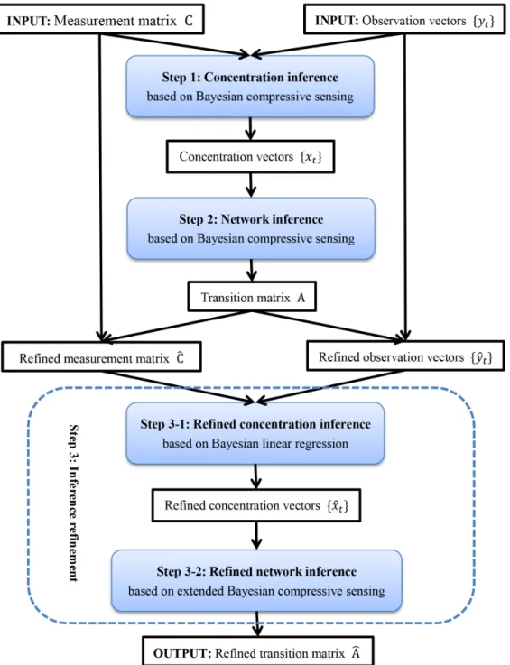
In this section, the core algorithm of CCELL, Bayesian compressive sensing, is first introduced. Then, we will explain the three sequential steps of CCELL: concentration inference, network inference and inference refinement. The structure of CCELL is detailed in Figure 1.
Bayesian compressive sensing
Bayesian compressive sensing, introduced by Ji, Xue and Carin [31], is a probabilistic version of compressive sensing based on the relevance vector machine [30]. Letwbe the signal of interest that is represented using aN-dimensional column vector. The sparsity of a vector is the proportion of (approximate) zero elements. A vector is sparse if its sparsity is greater than a threshold (usually 80%). A measurement matrixWis aM|N-dimensional matrix, whereMis the number of measurements. Typically,M is far less thanN. Each row ofWis a measurement vector, which is aN -dimensional row vector. A measurement is to obtain the inner product of the signal vector and a measurement vector. For example, a measurement vector (i.e. a row of the measurement matrix) is (0,1,0,1,0) and the signal vector is (1,10,100,1000,10000)0. The prime symbol0means the transpose of a vector or a matrix. The result of this measurement is the sum of the second and fourth elements, which is1010. An observation vectorgisM-dimensional column vector, each element of which represents a measurement result of the corresponding measure-ment vector. Assuming the measuremeasure-ment noises are independent additive white Gaussian with mean0and the covariance matrix s2I, we can get a system of linear equations as follows:
g~WwzN(0,s2I)
The symbol I denotes an identity matrix. For simplicity, the dimension ofIis various according to different equations without notation in this paper. Equation 1 is usually underdetermined, because the number of measurements M is far less than the number of elements of the signal vector N. However, the additional assumption that the signalwis sparse makes Equation 1 solvable. Bayesian compressive sensing is an inference algorithm to solve Equation 1 using a sparse prior distribution, which is typically Student’s t-distribution. Its input is an observation vectors
gand a measurement matrixW. The corresponding output is a distribution of the signalw.
Bayesian compressive sensing is an EM style iterative algorithm. Given a hyperparameter vectorbof the signalw, the E-step is to infer a posterior distribution of the signalw. The posterior is a multivariate Gaussian distribution with the mean vectormw and the covariance matrixSw as follows:
Figure 1. The workflow of CCELL.The CCELL method consists of 3 steps: concentration inference, network inference and inference refinement (including refined concentration inference and refined network inference). The core algorithm of the first two steps is Bayesian compressive sensing. The two substeps in Step 3 are based on Bayesian linear regression and extended Bayesian compressive sensing respectively. The input of CCELL is a measurement matrixCand its corresponding observation vectorsytthat are time-series generated by immunoprecipitation assays. The output of CCELL is a refined transition matrixAA^representing the cell-scale signalling network.
S{1w ~diag(b)zs {2
W0W ð2Þ
mw~s{2
SwW0g ð3Þ
wherediag(b)represents a diagonal matrix whose diagonal is the hyperparameter vector b. The M-step, based on the variational method[32], is to calculate an approximately optimal hyperpara-meters vectorbusing the posterior ofwcalculated in the previous E-step as follows:
b{ k ~S
kk
w zmw2 ð4Þ wherebkandmw denote thekth element of the hyperparameter vectorband the mean vectormwrespectively;Skk
w represents the element in the row and column of the covariance matrix Sw.
Before the execution of the Bayesian compressive sensing algorithm, the hyperparameter vector is often set to a random or given value. Then, a posterior distribution of the signal is inferred by the E-step. Subsequently, the M-step update the hyperpara-meter vector based on the mean vector and the covariance matrix of the posterior distribution inferred in the previous E-step. Afterwards, the updated hyperparameter vector is used to infer a new posterior distribution in the E-step of the next iteration. The Bayesian compressive sensing algorithm iteratively executes the E-step and M-E-step until stop conditions are satisfied.
According to the workflow in Figure 1, the Bayesian compres-sive sensing algorithm is used in the concentration inference and network inference steps. This is because that both of the two steps aiming at solving systems of linear equations with sparse constraints, which have identical forms with Equation 1. Bayesian compressive sensing can directly solve these systems of linear equations. More specifically, in Figure 1 the concentration vector yt, the measurement matrix C and the output concentration vector xt in Step 1 correspond to the observation vector g, the measurement matrix W and the signal vector w in Equation 1 respectively. Similarly, in Step 2 concentration vectors xt and
xt{1 at two consecutive time points correspond to the observation vectorg and the measurement matrix W, while the transition matrixArefers to the signal vectorwin Equation 1.
Step 1: Concentration inference
Mathematically, combined-measurements are modelled as a system of linear equations:
yt~CxtzN(0,s2mI): ð5Þ xt is a concentration vector. Each element of xt represents the concentration of a species at timet, which is an unknown variable to be inferred. The dimension of xt equals to the number of species in the network, denoted asN.Cis a measurement matrix that is given in advance. Each row ofCrepresents a combined-measurement. The dimension of C is M|N, where M is the number of measurements andNis the number of species.ytis an observation vector. Each element of yt represents the observed value of a measurement at time t. The dimension of yt is the number of measurements M. The random vector N(0,s2
mI) is measurement noises with mean0and the covariance matrixs2
mI. The variation of concentrations xt is defined as the difference between the concentration vectors at two adjacent time points:
Dxt~xt{xt{1: ð6Þ
Similarly, the variation of observations is defined as the difference between observation vectors at two adjacent time points:
Dyt~yt{yt : ð7Þ
The sparsity of variations is defined as the ratio between the number of time-invariant species and the number of all species. This definition is consistent with the definition of sparsity for a vector. According to the observation that the concentrations of only a few species in a cellular system vary significantly over a specific timescale, variations of concentrations are sparse. There-fore, Bayesian compressive sensing can be used to infer variations of concentrations by solving the following system of linear equations:
Dyt~CDxtzN(0,2s2mI): ð8Þ
In wet lab experiments, a cell is perturbed from its steady state by triggers. As a large fraction of species at steady state have zero concentrations [3], the initial concentrations of all species can be inferred by Bayesian compressive sensing directly. Therefore, it is assumed that initial concentrations are known in this paper. Concentration vectorxt at other time points can be calculated according to Equation 6.
Step 2: Network inference
This paper focuses on the biological networks that can be modelled by a system of linear equations:
xt~Axt zN(0,s2sI): ð9Þ Ais a transition matrix, whose elements are unknown variables to be inferred. The dimension ofAisN|N, whereN denotes the number of species. N(0,s2sI) is system noises with mean 0 and covariance matrix s2
sI. The networks modelled by differential equations can be also approximated by linear equations. One method is to define the transition matrix as a function of time, which can be calculated according to Jacobian matrices of the transition function [10]. The other method is to view higher order derivatives of concentrations as first order variables [22].
According to Equation 9, the jth row of A, a0
j, satisfies the following equation:
½xj2,xj3,:::,x
j T
0
~½x1,x2,:::,xT 0
ajzN(0,s2sI) ð10Þ where xjt denotes the jth element of concentration vector xt. Equation 10 is only for the time-series profile of species under one perturbation. It can be easily extended to any number of perturbations by successively combining all profiles together. Equation 10 can fit the form of Equation 1. The transpose of the jth rowa0
jis the signal to be inferred. The matrix ½x1,x2,:::,xT 0
and column vector½xj2,xj3,:::,x
j T
0
can be viewed as a measurement matrix and the corresponding observation vector respectively. According to a widely accepted assumption that structures of biological networks are usually sparse [3,33,34], Bayesian
com-1
,k
,k
kth kth
∆
{1
{1
{1
pressive sensing can be directly used to solve Equation 10. Thus, a posterior of thejth row of the transition matrix Ais calculated. Other rows can be independently inferred in a same way.
Step 3: Inference refinement
Structural indicator. For an inferred transition matrix AA~ outputted by Step 2, the structural indicator is defined as follows:
S(i,j,E)~ 1, jAA~ijj
§E
0, otherwise (
ð11Þ
whereAA~ij represents the inferred value of the element inith row and jth column of matrix AA~; E is a threshold parameter. If
S(i,j,E)~1, there is a link from species j to i over the predetermined timescale of experiments. If a species has no links with other species, it is called as a silent species over the timescale; otherwise, it is called as an active species. It is noteworthy that a time-invariant species can be an active species, such as an enzyme that catalyses other species without changing its concentration. The process of refinement is to remove silent species in order to formulate a small scale inference problem, which is detailed in Figure 2.
Refined concentration inference. All silent species over the
predetermined timescale are removed. The refined concentration
vector,^xxt, only contains the concentrations of active species. Each element of^xxt represents the concentration of an active species at timet, which is an unknown variable to be inferred. The refined measurement matrixCC^is derived fromCby removing all columns associated with silent species. An element of the refined measurements^yyt are calculated by subtracting concentrations of silent species involved in this measurement. Thus, the refined measurement model is as follows:
^
y
yt~CC^^xxtzN(0,s2mI): ð12Þ
It is noteworthy that the variations ofxx^t are not sparse. The assumptions of Bayesian compressive sensing are not satisfied. Instead, Bayesian linear regression is used to infer the posterior distribution of xx^t. The posterior is a multivariate Gaussian distribution with the mean vectorm^xxt and the covariance matrix S{1
^
x
xt as follows:
S{1
^
x xt ~SS
{1
^
x xt zs
{2 m CC^
0
^
C
C ð13Þ
mxxt^~S^xxt(SS{1
^
x xt mm^xxtzs
{2 m CC^
0
^
y
yt) ð14Þ
Figure 2. The process of refinement.The equations at the left and right side of arrows are original and reduced respectively. According to inferred transition matrixAA~, there are two pathway and crosstalk between them. The4th, 5th, 6th, 7th, 11th, 12th, 13th, 14th, 15th species are silent, having no links with others. All elements associated with the silent species are removed from the transition matrixAto form the refined transition matrixAA^. All columns measuring the silent species are deleted from the measurement matrixCto form the refined measurement matrixCC^. The refined concentration vector,xx^, only keeps the concentrations of active species (e.g.,1th, 2th, 3th,8th,9th,10th). An element of the refined observation vector^yyis equal to the corresponding element of the observation vectorysubtracted by the concentrations of the silent species involved in this measurement. If all species involved in a measurement are silent, simply remove this measurement.
doi:10.1371/journal.pone.0095326.g002
wheremm^xxtandSS^xxtare the mean vector and the covariance matrix of the prior distribution of^xxtrespectively. The prior distribution of
^
x
xtcan be calculated using the results of Step 1.
Refined network inference. All elements associated with
silent species are removed from the transition matrixAto form the refined transition matrixAA^. Therefore, the refined system model is as follows:
^
x
xt~AA^^xxt{1zN(0,s2sI): ð15Þ
Although the refined transition matrixAA^is sparse, it cannot be inferred by Bayesian compressive sensing directly. This is because
Table 1.Characteristics of the benchmark network set.
ID Components
# species
#time-variant
species #links
n-4 JAK-STAT 300 4 4
n-11 ERK 300 11 20
n-39 p38 300 39 61
n-50 ERK and p38 300 50 83
n-53 GR, ERK and p38 300 53 93
n-58 GR, JAK-STAT, ERK and p38 300 58 101
doi:10.1371/journal.pone.0095326.t001
Figure 3. Boxplots of RMSE of inferred concentrations.The 6 subplots depict the results of applying inference method to 6 benchmark networks. For each network, its inference results under different numbers of perturbations, varying from 2 to 7, are shown individually. The median values of RMSE approximate to 0 and the3rd quartile values range from 0.0031 to 0.011.
doi:10.1371/journal.pone.0095326.g003
Figure 4. ROC curves of network structure inference.The performance of structure inference, under 6 different numbers of perturbations (from 2 to 7), is evaluated by ROC curves. Each subplot contains the inference results for 6 benchmark networks. The average AUROC is 0.97. More specifically, the maximum AUROC value 1.0 is achieved by the n-4 network (3–7 perturbations) and the n-11 network (6–7 perturbations), while the minimum AUROC value 0.88 is obtained by the n-58 network (2 perturbations).
Bayesian linear regression infers a distribution of^xxtrather than a specific value. If we would like to apply Bayesian compressive sensing to infer the distribution of^aaj, then only the mean ofxx^t distribution is used for calculation. In this case some information is ignored. Thus, we extend Bayesian compressive sensing to extract information from distributions not just from their mean.
The E-step of the extended Bayesian compressive sensing infers a posterior distribution of^aa0j, which represents the jth row ofAA^, from the posterior distributions of the concentrations ^xx. The posterior is a multivariate Gaussian distribution with the mean
vectorm^aaj and the covariance matrixS{
^
a
aj as follows:
S{1
^
a
aj ~diag(bj)zs {2 s
XT
t~1
v^xxtxx^0tw ð16Þ
m^aaj~s{2s S^aaj XT
t~2
v^xxt{1xx^jtw ð17Þ
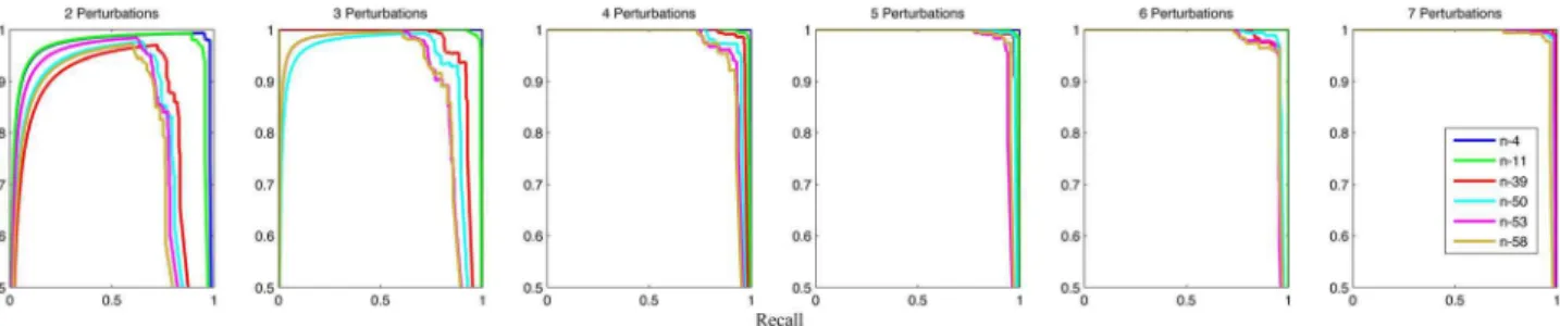
Figure 5. Precision-recall curves of network structure inference.The performance of structure inference, under 6 different numbers of perturbations (from 2 to 7), is evaluated by Precision-recall curves. Each subplot contains the inference results for 6 benchmark networks. The average AUPR is 0.95. More specifically, the maximum AUPR value 1.0 is achieved by the n-4 network (3–7 perturbations) and the n-11 network (6–7 perturbations), while the minimum AUPR value 0.75 is obtained by the n-58 network (2 perturbations).
doi:10.1371/journal.pone.0095326.g005
Figure 6. Sensitivity/specificity v.s. threshold parameter.These graphs show the relationships between sensitivity (above) and specificity (below) and threshold parameterEfor 6 different benchmark networks with different numbers of perturbations varying from 2 to 7. ForE~0, the average specificity is 0.9989 and the average sensitivity reaches its maximum value of 0.9453. WhenEincreases to0:2, the average specificity is 0.9999 and the average sensitivity decreases to 0.8742. IfEincreases to a relatively large value0:6, the average specificity achieves 1.000 but the average sensitivity becomes 0.8188.
doi:10.1371/journal.pone.0095326.g006
where we have:
v^xxt^xx0tw~v^xxtwv^xx0twzCov(^xxt,^xx
0
t): ð18Þ
bj denotes the hyperparameter of ^aaj. diag(bj) represents a diagonal matrix whose diagonal is vectorbj. The angled brackets
v:wdenote the expectation of a distribution.Covrepresents the covariance of two random variables.
The M-step of the extended Bayesian Compressive sensing, which is identical to Bayesian compressive sensing, aims to calculate approximately optimal hyperparameters using the variational method [32] as follows:
b{jk1~Skk
^
a aj zm^aaj
2
: ð19Þ
Results
A set of benchmark cell-scale networks is designed to demonstrate our method. Each cell-scale network contains 300 species, while only a fraction of species are time-variant over the investigated timescale. The dynamics of these networks are modelled using systems of linear functions. The dimensions of the transition matrices are300|300. For a time-invariant species j, the elements of jth row in the transition matrix are all zero except thejth element having the value of1; for a time-variant species, its corresponding row has more than one non-zero elements to represent its interactions with other species in the network.
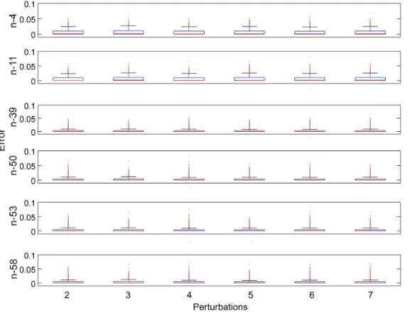
The set of benchmark cell-scale networks has varying numbers of variant species. The rows of transition matrices for time-variant species are constructed by taking the structures of4 well-studied signalling pathways: JAK-STAT [2], GR [35], ERK [1], Figure 7. Bar charts of RMSE for inferred transition matrices.These charts show the results of both Step 2 and Step 3 for 6 different benchmark networks with different numbers of perturbations varying from 2 to 7. In Step 2, the RMSE values range from1:9|10
{6
to2:1|10 {2 with the mean value of6:2|10
{
; in Step 3, the RMSE values range from1:6|10 {
to5:9|10 {
with the mean value of1:3|10
{3. The RMSE ratios (Step 3/Step 2) vary from 0.14% to 51% with the mean value of 17%.
doi:10.1371/journal.pone.0095326.g007
3
3 7
p38 [3], and crosstalk amongst them [5,6,35]. Details of the benchmark set are listed in Table 1.
In order to study the effect of perturbations, where various doses or types of inhibitors/stimuli perturb the initial state of the network, different numbers of perturbations are used to simulate benchmark networks. In our simulation, we check the perfor-mance of CCELL with the number of perturbations varying from 2 to 7 as these values are frequently used in wet-lab experiments. Under each perturbation, the initial concentration of each species is randomly generated from a normal distribution with mean of 100, standard deviation of30. Concentrations of 300 species at 5 sequential time points are generated using benchmark network model and corresponding initial state. For each time point, 150 combined-measurements are carried out according to a predefined measurement matrix. The measurement matrix is generated using low-density parity-check code [36]. Our experiments only focus on investigating the performance of our method when both system noises and measurement noises are maintained at small level (standard deviation~0:01). The code and benchmark network set are available at http://dsg.doc.ic.ac.uk/publications/ccell/.
Figure 3 depicts RMSE values of inferred concentrations for the 6 benchmark networks under 6 different numbers of perturba-tions. RMSE values in Figure 3 are calculated using differences between inferred concentrations and true concentrations. Almost all RMSE values are below 0.05, except some outliers. Most of the RMSE values are in the range between 0 and 0.011. This indicates that our method accurately and stably infers the concentrations. It can be clearly observed that the RMSE values are not influenced by the number of perturbations, which is consistent with the principle of our method that concentrations of each time point are inferred independently. As can be seen in Figure 3, there are no
significant differences between the RMSE values of different benchmark networks. However, the RMSE values of the two networks with high sparsity of variations, n-4 and n-11, are slightly greater than the other three networks. This might be because prior distributions of Bayesian compressive sensing are not sparse enough.
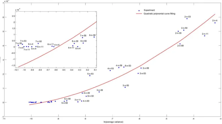
After obtaining the inferred transition matrixAA~ of a network in Step 2, the structure of the network is calculated using structural indicatorS(i,j,E)according to Equation 11. A link from speciesjto iare inferred, if S(i,j,E)= 1. Varying the threshold parameterE results in different structures. To show the performance of inferring real links in the target networks, ROC and Precesion-recall curves of 6 benchmark networks under 6 different numbers of perturbations are drawn in Figure 4 and Figure 5 respectively. An inferred link is true positive, if it does exist in the network; otherwise, it is false positive. The average of all AUROC and AUPR values is as high as 0.97 and 0.95 respectively, which demonstrates the effectiveness of our method. As evident from Figure 4 and Figure 5, the AUROC and AUPR values rise up as the number of perturbations increases. This indicates that adding new perturbations is an effective way to boost the performance of structure inference. The sparsity of variations is another factor to affect the performance. The AUROC and AUPR values positively correlate with the sparsity of variations. Figure 6 demonstrates relationships between sensitivity or specificity and threshold parameter E for 6 different benchmark networks with different numbers of perturbations varying from 2 to 7. WhenEincreases from0to0:2, the average sensitivity falls from0:9453to0:8742 and the average specificity maintains close to 1. The decrease of the average sensitivity is significant, while the change of the average specificity is negligible. The stability of the average Figure 8. Relationship between the average variance and RMSE.Each point represents an experiment for a benchmark network under a specific number of perturbations. For example, 2-n-53 means the experiment for n-53 network under 2 perturbations. The x-coordinate indicates the natural logarithm of the average variance for all elements in the refined transition matrix, while the y-coordinate indicates the RMSE values of the refined transition matrix. The RMSE values range from1:6|10
{7to5
:9|10
{3and the average variance varies from4
:2|10 5
{
to4:0|10 2 {
specificity is caused by high sparsity of cell-scale signalling networks. Thus, we fix E to be 0 in the following experiments. For simplicity, we suggest that except special conditions users should setEto be 0 for sparse networks.
Figure 7 illustrates the RMSE values of transition matrices inferred by both Step 2 and Step 3 for 6 benchmark networks under 6 different numbers of perturbations. RMSE values in Figure 7 are calculated using differences between the elements of the inferred transition matrix and the corresponding elements of true transition matrix. Step 2 infers the transition matrices of a whole network, while Step 3 only infers transition matrices of a refined network only containing active species. In Step 3, the threshold parameterEis chosen to be 0. In order to fairly compare the results of Step 2 and Step 3, RMSE values in Figure 7 only calculate the errors in refined transition matrices. Similar to AUROC values, the RMSE value correlates with the number of perturbations and the sparsity of variations. The correlation between the RMSE value and number of perturbations is much stronger than the correlation between the RMSE value and sparsity of variations. It can be seen in Figure 7 thatz the RMSE value decreases significantly to a stable and small value as the number of perturbations increases. The number of perturbations required to reach a stable RMSE value varies across different networks with various sparsity of variations. For the results of Step 3, the n-4 network only needs 3 perturbations, while the n-39 network requires 5 perturbations. It is visible that the convergence rate of results of Step 3 is higher than that of Step 2. What’s more, the RMSE values of Step 3 are always smaller than those of Step 2. The RMSE ratios (Step 3/Step 2) vary from 0.14% to 51% with the mean value of 17%, which demonstrates Step 3 substantially improves the performance of transition matrix estimation. It is also
clear that Step 3 is more robust than Step 2 under varying number of perturbations.
Figure 8 shows the relationship between the average variance for all elements of the inferred transition matrix according to Equation 16 and their RMSE values. The RMSE values range from1:6|10
{7to5
:9|10
{
, while the average variance varies from 4:2|10
{
to 4:0|10
{
. As illustrated by Figure 8, the RMSE value and the average variance have strong correlation that can be well fitted by a quadratic curve, having the Spearman’s correlation coefficient to be 0.94. Thus, the average variance is a promising way to represent the accuracy of the inference results when RMSE cannot be calculated due to the unavailability of the real transition matrix. One potential usage of average variance is to adjust the threshold parameter E. Specifically, when we get different inference results using differentE, we can choose the most appropriateEvalue which results with lowest average variance.
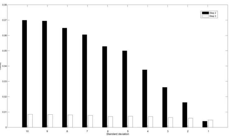
We stress that the promising results obtained in the above experiments are conditioned on stringent constraints of noises. To investigate the performance of our method in the presence of significant noises, the noises are set to be higher than those in previous experiments. That is, the standard deviations of noises vary from 10 to 1 (signal mean is 100). For n-39 network under 6 perturbations, Figure 9 reveals the relationship between noise levels and the RMSE values of transition matrices inferred by both Step 2 and Step 3. The RMSE values of Step 3 can be always achieved larger or close to those obtained in Step2. The RMSE values of both steps gradually decline with the reduced noise levels. The RMSE values of Step 2 have been decreased by 94%, while the decrease for Step 3 is 44%.
Figure 9. Relationship between noise levels and RMSE.This chart shows the RMSE values for inferred transition matrices of n-39 network under 6 perturbations at different noise levels. The standard deviations of noises vary from 10 to 1. In Step 2, the RMSE values range from7:0|10
{2 to4:0|10
{3
; in Step 3, the RMSE values range from8:5|10 3 {
to4:7|10 3 {
. doi:10.1371/journal.pone.0095326.g009
3
ity. To the best of our knowledge, CCELL is the first attempt to infer cell-scale signalling networks from a holistic perspective by exploring separation of timescales and cross-reactivity. We demonstrate that CCELL is effective for inferring benchmark cell-scale networks without structure constraints. Instead of exhaustively measuring all individual species, we show that M combined measurements are sufficient to infer the network model with acceptable accuracy, whereMequals to the half of the total number of species in the network.
This paper models biological networks as linear dynamical systems. A classical algorithm to infer the parameters of a linear dynamical system is the expectation maximization (EM) algorithm. The E-step is to infer a distribution of hidden variables (concentrations) using the forward-backward algorithm based on current estimates of parameters. The M-step is to update parameters based on the distribution of hidden variables inferred in the E-step. The E-step and M-step are executed in an iterative way. An advantage of the forward-backward algorithm is that it uses the transition matrix of two adjacent time points of hidden variables to boost the accuracy of hidden variables. However, the transition matrix inferred in M-step is not very accurate, especially when observed data is scarce, while the forward-backward
inferring cell-scale signalling networks over a predetermined timescale. By repeating the measurement and inference proce-dures over different timescales, multiple timescale-specific network models can be obtained. How to integrate them into a unified whole is itself an attractive problem.
CCELL is a promising routine to reveal the mechanism of a complex cellular signal transduction system from a holistic perspective. The current situation, where cell-scale signal trans-duction models are rarely built due to its difficulty, may be changed. Signalling network databases can be built more efficiently by incorporating much more cell level models to comprehensively understand complex biological processes. Better understanding of complex biological processes is fundamental to understand life and design drugs.
Author Contributions
Conceived and designed the experiments: LN XY IA ZX YG. Performed the experiments: XY. Analyzed the data: LN XY YG. Contributed reagents/materials/analysis tools: XY. Wrote the paper: LN XY IA ZX YG. Supervised the project: YG.
References
1. Kolch W (2000) Meaningful relationships: the regulation of the ras/raf/mek/erk pathway by protein interactions. Biochemical Journal 351: 289–305. 2. Swameye I, Mu¨ller T, Timmer Jt, Sandra O, Klingmu¨ller U (2003)
Identification of nucleocytoplasmic cycling as a remote sensor in cellular signaling by databased modeling. Proceedings of the National Academy of Sciences 100: 1028–1033.
3. Hendriks BS, Hua F, Chabot JR (2008) Analysis of mechanistic pathway models in drug discovery: p38 pathway. Biotechnology Progress 24: 96–109. 4. Bonifacino JS, Dell’Angelica EC, Springer TA (2001) Immunoprecipitation.
Current Protocols in Immunology 41: 8.3.1–8.3.28.
5. Shuto T, Imasato A, Jono H, Sakai A, Xu H, et al. (2002) Glucocorticoids synergistically enhance nontypeablehaemophilus influenzae-induced toll-like receptor 2 expression via a negative cross-talk with p38 map kinase. Journal of Biological Chemistry 277: 17263–17270.
6. Wang Z, Yang H, Tachado SD, Capo´-Aponte JE, Bildin VN, et al. (2006) Phosphatase-mediated crosstalk control of erk and p38 mapk signaling in corneal epithelial cells. Investigative Ophthalmology & Visual Science 47: 5267–5275. 7. Junttila MR, Li SP,Westermarck J (2008) Phosphatase-mediated crosstalk between mapk signaling pathways in the regulation of cell survival. The FASEB Journal 22: 954–965.
8. Guo X,Wang XF (2009) Signaling cross-talk between tgf-b/bmp and other pathways. Cell Research 19: 71–88.
9. Kreeger PK, Lauffenburger DA (2010) Cancer systems biology: a network modeling perspective. Carcinogenesis 31: 2–8.
10. Sontag E, Kiyatkin A, Kholodenko BN (2004) Inferring dynamic architecture of cellular networks using time series of gene expression, protein and metabolite data. Bioinformatics 20: 1877–1886.
11. Schmidt H, Cho KH, Jacobsen EW (2005) Identification of small scale biochemical networks based on general type system perturbations. FEBS Journal 272: 2141–2151.
12. Mendes P, Kell DB (1998) Non-linear optimization of biochemical pathways: applications to metabolic engineering and parameter estimation. Bioinformatics 14: 869–883.
13. Quach M, Brunel N, d’Alche´ Buc F (2007) Estimating parameters and hidden variables in non-linear state-space models based on odes for biological networks inference. Bioinformatics 23: 3209–3216.
14. Sun X, Jin L, Xiong M (2008) Extended kalman filter for estimation of parameters in nonlinear state-space models of biochemical networks. PloS ONE 3: e3758.
15. Toni T, Welch D, Strelkowa N, Ipsen A, Stumpf MP (2009) Approximate bayesian computation scheme for parameter inference and model selection in dynamical systems. Journal of the Royal Society Interface 6: 187–202. 16. Yang X, Guo Y, Guo L (2013) An iterative parameter estimation method for
biological systems and its parallel implementation. Concurrency and Compu-tation: Practice and Experience.
17. Manning G, Whyte DB, Martinez R, Hunter T, Sudarsanam S (2002) The protein kinase complement of the human genome. Science 298: 1912–1934. 18. Forrest AR, Ravasi T, Taylor D, Huber T, Hume DA, et al. (2003)
Phosphoregulators: protein kinases and protein phosphatases of mouse. Genome Research 13: 1443–1454.
19. Hecker M, Lambeck S, Toepfer S, Van Someren E, Guthke R (2009) Gene regulatory network inference: data integration in dynamic models - a review. Biosystems 96: 86–103.
20. Choudhary C, Mann M (2010) Decoding signalling networks by mass spectrometry-based proteomics. Nature Reviews Molecular Cell Biology 11: 427–439.
21. Dunn JD, Reid GE, Bruening ML (2010) Techniques for phosphopeptide enrichment prior to analysis by mass spectrometry. Mass Spectrometry Reviews 29: 29–54.
22. Xiong H, Choe Y (2008) Structural systems identification of genetic regulatory networks. Bioinformatics 24: 553–560.
23. Papin JA, Palsson BO (2004) The jak-stat signaling network in the human b-cell: an extreme signaling pathway analysis. Biophysical journal 87: 37–46. 24. Bhalla US, Iyengar R (1999) Emergent properties of networks of biological
signaling pathways. Science 283: 381–387.
25. Weng G, Bhalla US, Iyengar R (1999) Complexity in biological signaling systems. Science 284: 92–96.
26. Frank SA (2002) Chapter 4: specificity and cross-reactivity. In: Immunology and Evolution of Infectious Disease, Princeton University Press.
27. Cande`s EJ, Romberg J, Tao T (2006) Robust uncertainty principles: exact signal reconstruction from highly incomplete frequency information. IEEE Transac-tions on Information Theory 52: 489–509.
28. Donoho DL (2006) Compressed sensing. IEEE Transactions on Information Theory 52: 1289–1306.
30. Tipping ME (2001) Sparse bayesian learning and the relevance vector machine. The Journal of Machine Learning Research 1: 211–244.
31. Ji S, Xue Y, Carin L (2008) Bayesian compressive sensing. IEEE Transactions on Signal Processing 56: 2346–2356.
32. Bishop CM, Tipping ME (2000) Variational relevance vector machines. In: Proceedings of the Sixteenth Conference on Uncertainty in Artificial Intelligence. Morgan Kaufmann Publishers Inc., pp. 46–53.
33. August E, Papachristodoulou A (2009) Efficient, sparse biological network determination. BMC Systems Biology 3: 25.
34. Yeung MKS, Tegne´r J, Collins JJ (2002) Reverse engineering gene networks using singular value decomposition and robust regression. Proceedings of the National Academy of Sciences 99: 6163–6168.
35. Necela BM, Cidlowski JA (2004) Mechanisms of glucocorticoid receptor action in noninflammatory and inflammatory cells. Proceedings of the American Thoracic Society 1: 239–246.