Determinants of Foreign Direct Investment in Romania: a Quantitative Approach

DETERMINANTS OF FOREIGN DIRECT INVESTMENT IN ROMANIA:

A QUANTITATIVE APPROACH

Calcedonia Enache

1*

_{and Fernando Merino}

2

1)

University of Agronomic Sciences and Veterinary Medicine, Bucharest, Romania

2)

University of Murcia, Murcia, Spain

Please cite this article as:

Enache, C. and Merino, F., 2017. Determinants of Foreign Direct Investment in Romania: a Quantitative Approach. Amfiteatru Economic, 19(44), pp. 275-287

Article History

Received: 26 September 2016 Revised: 18 November 2016 Accepted: 17 December 2016

Abstract

This study aims to examine the dynamic relationship between foreign direct investments (FDI) and economic growth, using the Structural Vector Autoregressive model, in the period 2007-2014. The results of the econometric model show that the trajectory of FDI has its own origins, with reduced influences from economic growth. Another important conclusion is that there is a unidirectional causal relationship from the economic growth towards FDI, more precisely the influence of FDI on economic growth does not have a systematic, anticipatory nature. These results were achieved in the condition that, in the analyzed period, the net inflows of FDI were influenced by the lack of certainty on the sustainable re-launching of the economic growth both domestically and internationally, the segmentation of the financial market, the domestic structural reforms.

Keywords: foreign direct investment, economic growth, vector autoregressive model, Sims-Bernanke decomposition, Granger causality test

JEL classification: C180; E430; F21

Introduction

Foreign direct investments (FDI) play an important role in the Romanian economy, perceived as a factor that boosts economic growth, a supplement of local investment and an important financier of the current account deficit. In addition, they carry technological flow vectors, with influence on the productivity, employment and profitability of domestic companies.

The net inflows of FDI accounted for 6.3 percent of GDP in 2008, 0.8 percentage points higher than the previous year. The growth was mainly duethe capital increases performed at a series of companies which were stimulated by the effects of the full capital account liberalisation and the introduction of the flat corporate income tax. In a global environment dominated by uncertainties and major risks, the share in the GDP of the net inflows of FDI

ranged from 2.8 percent in 2009, followed by a downward trend over the next two years, to 1.3 percent. The increase of the share of the short term foreign debt in the total foreign debt from 19.2 percent in 2009 to 23.1 percent in 2011, accompanied by an unpredictable fiscal regime represented an appreciable source of instability for the Romanian economy, which in some cases resulted in the restriction or cessation of the activities initiated by foreign investors. Later, in the period 2012-2014, the net inflows of FDI fluctuated at around 1.9 percent GDP, while the relatively high volume of international reserves helped to increase Romania's credibility abroad. Thus, the forex reserve registered an average annual growth rate of 3.2 percent, covering six months of future imports of goods and services at the end of 2014, which favoured a stable exchange rate for the RON / EUR, with a significant contribution to lowering the annual inflation rate and ensuring financial stability. In 2014, the net inflows of FDI were directed mainly to the manufacturing industry (38.4 percent of the total), real estate transactions (13.7 percent), constructions (13.0 percent), information technology and communications (10.5 percent). The main origin of foreign inflows was the Netherlands, Austria, Germany, Cyprus and France.

From a microeconomic point of view, the relevance of these figures is even clearer. Since 1997, the net inflows of FDI have been an important change factor in Romanian firms (Hunya, 2002).According to the statistics analysed by the National Bank of Romania, in 2014 the companies that received flows as FDI created approximately 50.0 percent of the value added by non-financial companies, accounted for 24.9 percent of the number of employees in the economy, with a contribution of 70.9 percent on exports of goods and 64.7 percent of imports of goods. For this category of companies, the return on equity was maintained during the period 2011-2014 in the range of 9.1-12.1 percent, while at the level of non-financial companies this indicator was in the range of 8.2-11.2 percent. In 2014, the degree of indebtedness was at 2.3 compared to 2.5 in 2013 and 1.5 in 2011. In August 2014, the non-performing loans ratio was of 15.7 percent, 6.3 percentage points below the average on economy. Then, given the importance of these companies in the Romanian economy, the study of FDI inflows is an interesting topic that deserves further research.

This study aims to examine the dynamic relationship between FDI and economic growth in recent years. This is a hot topic in the analysis of FDI, since as UNCTAD (2016) reports, in the last years FDI flows have a lower growth impact since a large part are attributed to corporate reconfiguration more than greenfield investments.

It must be noted that the studied period (2007-2014) is characterised by a deep financial crisis that reduced FDI flows worldwide from USD 1902 billion in 2007 to USD 1277 billion according to UNCTAD. Different explanations have been signalled for this reduction, but as UNCTAD (2010) explains, the lack of funding for this main investors, the turmoil in financial markets that obscures price signals which are determinants on the decision to invest may explain the reduction in the worldwide FDI flows. Then, an analysis of this period, different than Misztal (2010) will help to know the role of FDI in a completely different economic situation.

modelling (Păuna, 2007). The VAR techniques can be applied only to stationary series (Albu et al., 2003). The main purpose of the VAR analysis is to evaluate the effects of various shocks on the variables of the system. Each variable is affected by its own innovations, and the innovations in the other variables (Boţel, 2002).

The study has the following structure: Part Two reviews the specialized literature regarding the analysis of the relationship between FDI and economic growth. Part Three is dedicated to the VAR methodology. Part Four shows the time series used, the structure of the causal relationships between the variables and the modelling stages. Part Five contains the results from the econometric model and their interpretation. Part Six presents the final conclusions.

1. Literature Review

The analysis of the relationship between FDI and economic growth is a widely researched topic in the specialized literature. Studies in the field have shown that both developing countries and developed countries encourage the attraction of FDI, even though their objectives are diverse.

impact in the first two countries mentioned above. In completing the picture, the studies of the Keller and Yeaple (2009), Lipsey and Sjöholm (2004) show that FDI bring advanced technology and performant management to the host countries. In this context, the local companies, competing with the foreign ones, are forced to improve their business, either by observing and taking over technologies, organizational practices, strategies which are used by multinational companies (MNCs) (Blomstrom and Kokko, 1998), or by attracting employees trained by MNCs (Meyer, 2004; Spencer, 2008). According to Moran (quoted by Andrei, 2013), instead of connecting the value of the domestic currency resources to that of FDI, MNCs can crowd local producers out of business and replace the imports of raw materials. Moreover, Mencinger (2003), analysing the economies of 8 candidate countries to joining the European Union in the period 1994-2001, suggests that FDI negatively affect economic growth. In this regard, the author argues that, in case of the investigated countries, FDI had as main purpose the acquisition of fixed assets from the patrimony of public institutions and the revenues thus obtained did not finance productive investments and generate a growth in imports and thereby the current account deficits. In addition, Kholdy and Sohrabian (2005), Javorcik (2004), Grilli and Milesi-Ferretti (1995) consider that FDI do not affect economic growth.

When the connection between FDI and economic growth is studied, a notable problem is the potential endogeneity between them. Thus, on the one hand, the bilateral causality is tested and, on the other hand, a system of equations is estimated within which the equation associated with FDI may include variables such as economic growth, interest rates, foreign exchange, infrastructure.

Chowdhury and Mavrotas (2006) examine the connection between FDI and economic growth in Chile, Malaysia and Thailand in the period 1969-2000, using the long-run Granger causality test proposed by Toda and Yamamoto (1995). The results show that in Malaysia and Thailand there is a mutual causal relationship between the two variables, while in Chile a unidirectional causal relationship from growth to FDI was identified. Choe (2003), using a panel VAR model to examine the connection between FDI and economic growth in 80 developed and developing countries in the period 1971-1995, finds that there is a bidirectional causal connection between the studied variables, with clearer effects from growth to FDI. Later, Moudatsou and Kyrkillis (2011) studied the connection between FDI and economic growth both in developed EU countries and in some ASEAN developing countries, namely Indonesia, Singapore, Philippines and Thailand in the period 1970-2003, with the aid of the co-integration and error-correction technique. The authors reached the conclusion that FDI cause economic growth only in Finland and Indonesia, while in all the countries included in the analysis economic growth motivates FDI. In case of the Romanian economy, Misztal (2012) using a VAR model to assess the relationship between FDI and economic growth in the period 2000-2009, notes that FDI substantially influenced economic growth.

promotion of human capital and technical progress encourage the attraction of FDI, which drive economic development and competitiveness.

2. The model

Our objective is to use a model capable to identify the interactions between the macroeconomic variables. The theoretical model is similar to that presented by Enache (2005).

Yt is considered as a VAR model of p (VAR(p)) order in the form:

Yt = Щ1Yt-1+Щ2Yt-2+…+ЩpYt-p + et (1) where:

Yt is a (nx1) vector of endogenous variables;

Щi is (nxn) coefficient matrix, for

i

=

1

,

p

;

et is (nx1) vector of errors with M(et)=0 and the variance-covariance matrix M(etetT)=Σe. The VAR(p) process is stationary if the polynomial defined from determinant det(In-Щ1Z -…-ЩpZp) ≠ 0, for │z│≤1 has the roots outside the unit circle in the complex plane (Hamilton,1994).

Equation (1) can be written using the lag operator lag Lj_y

t =yt-j in reduced form, as follows:

(In – Щ1L – Щ2L2 – … – ЩpLp)Yt = et or: (2)

Щ(L)Yt = et (3) From the form of equation(1) unrestricted VAR we can obtain a VAR restricted equation (Pfaff, 2008):

ЩYt= Щ1*Yt-1+Щ2*Yt-2+…+Щp*Yt-p +Φut (4) where ut are the structural innovations, M(ut,utT)=Σu is the variance-covariance matrix, the coefficients of the Щi* matrix, for

i

=

1

,

p

are structural coefficients, that generally differ from their counterparts in reduced form, Φ is the diagonal matrix.

Multiplying equation(4) with Щ-1 _{we obtain:}

Yt= Щ-1(Щ1*Yt-1 + Щ2*Yt-2+…+ Щp*Yt-p+Φut) (5) Equation (5) can be re-written as:

Yt= Щ1Yt-1 + Щ2Yt-2+…+ ЩpYt-p+ vt 6) where vt=Щ-1Φut makes the connection between the two forms. The variance-covariance matrix is: Σv=Щ-1ΦΦTЩ-1

T .

In order to determine the structural innovations, the minimum k(k-1)/2 zero restrictions

must be set to the coefficients of the Щ matrix in equation (5)→The Щ matrix reveals the

interdependency connections between the variables included in the model. In this regard, the Sims-Bernanke decomposition (1986) can be used for short-term innovations, admitting

t p j j t j i t p i j

t a Z b Y u

Z 1

1 1 1

1

1

∑

∑

= − − = + + + =α t p j j t j i t p i j

t a Z b Y u

Y ₂

1 2 1

2

2

∑

∑

= − − = + + + =α

The results of the VAR model are:

•The impulse response function (IRF) examines the impact of an innovation of a standard deviation of the residuals of a variable on the future evolution associated with each

variable in the model. IRF is expressed by the relationship: _h

t h t

u

y

₌

_υ

∂

∂

₊

, where υ_ij, the

element of the υ_h matrix highlights the impact that the increase by one unit of the u_j,t variable at the time t has on the y_{t+h variable,} if the other variables in the system exert a constant action.

•The variance decomposition (VD) determines, by percentage, the specific weight in the variance of a variable that is the result of their own shock and of the shocks from the other variables in the system.

•The Granger causality test (1969) shows whether there is a statistical connection between the data sets of variables Y and Z.It can be said that Y Granger causes Z, whether a forecast of Z performed based on the past values of Z and Y is better than a forecast made only based on the values of Z in the previous period.The Granger causality test is based on the following regression equations:

(7)

(8)

that assumes that the errors, u_1tand u_2t, are uncorrelated

.

Testing the null hypothesis Y does

not Granger Cause Z, i.e. H0:

∑

=

=

p j j

b

1

1

0

, it is carried out using the F-test.

3. Data description, modelling

Economic literature has two different indicators for the size of an economy: GDP and GNP. While GDP measures the value of the production inside the country borders, GNP measures the value of the production of those economic agents that are resident in those countries. Obviously, the difference emerges from the fact that part of the production developed in the country is done by inputs which are no residents in the country (and reverse). Given the low value of the income of labour (this is trans-border workers) most of it comes from the income of foreign capitals invested in the country. GNP is usually preferred (see, for example the methodology of the Human Development Index, or the criteria for European Cohesion and Regional Funds), since it is a better proxy of the income available for the citizens of that country.

In order to highlight the reaction of the FDI to various innovations in the economy, we estimated a VAR model, using the quarterly data from the period 2007-2014.In this regard, we included the following variables in the model:

FDIG Net inflows of FDI (percent of GDP)

The data series were taken from periodicals of the National Bank of Romania. The data series for the FDIG and the RGNP were seasonally adjusted using the TRAMO/SEATS method. The Augmented Dickey – Fuller test (Dickey and Fuller, 1979) and the Kwiatkowski-Phillips-Schmidt-Shin test (Kwiatkowski, Phillips, Schmidt and Shin, 1992) reveal that the three variables are stationary (Table no. 1).

Table no. 1: Evaluation of the series integration order

Notes:The tests are performed for the series in levels. The tests contain constant, constant and trend. The series is stationary if the value obtained is less than at least one of the critical values in absolute value.

The choice of the optimum number of lags in order to estimate the VAR model was made using the Akaike (1974, 1976), Schwarz (1978) and Hannan-Quinn (1979) criteria. The Akaike and Hannan-Quinn criteria indicated 2 lags. Since the VAR is stable, and the tests carried out on the errors reveals that they are distributed normally, they are not heteroscedastic and auto correlated, we opted for the Schwarz criterion, who selected a period as optimum lag (Table no. 2).

Table no. 2: VAR lag order selection criteria

The structure of the causal relations between FDIG, RGNP and Pr is presented in Table no. 3.

Table no. 3: Щ matrix structure Variable Augmented Dickey – Fuller test

Kwiatkowski – Phillips – Schmidt – Shin test Specification t-Statistic Specification t-Statistic FDIG

RGNP Pr

c,t c c,t

-4.789 -3.065 -4.833

c c c

0.699 0.114 0.624

Test critical values 1 percent level 5 percent level 10 percent level

MacKinnon (1996) c c,t -3.7 -4.3 -3.0 -3.6 -2.6 -3.2

Kwiatkowski-Phillips-Schmidt-Shin (1992) c

0.7 0.5 0.3

Lag LogL LR FPE AIC SC HQ

0 136.2033 NA 1.48e-08 -9.514524 -9.371788 -9.470888

1 211.1540 128.4868 1.34e-10 -14.22528 -13.65434* -14.05074

2 225.7799 21.93887* 9.21e-11* -14.62713* -13.62798 -14.32168*

3 229.8270 5.203386 1.40e-10 -14.27335 -12.84599 -13.83700

4 242.9162 14.02423 1.19e-10 -14.56545 -12.70988 -13.99818

* indicates lag order selected by the criterion

LR: sequential modified LR test statistic (each test at 5% level) FPE: Final prediction error

AIC: Akaike information criterion SC: Schwarz information criterion HQ: Hannan-Quinn information criterion

FDIG RGNP Pr

FDIG 1 1 1

RGNP 0 1 0

The imposed restrictions show that over a quarter, the FDIG are influenced by the RGNP and Pr, while the latter responds to the developments in the RGNP. In addition, each variable is influenced by itself.

4. Estimates and results

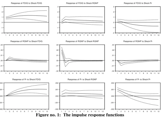
The impulse response functions to an innovation in the three series, simulatedon the basis of the estimated model, are shown in Figure no. 1.

Figure no. 1: The impulse response functions

The reaction of FDIG is strong to its own shocks, after the first 7-8 quarters remaining at a high level. FDIG respond positively to the shocks in the RGNP, peaking in quarter 2, following a period of gradual reduction in their intensity. In addition

,

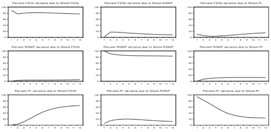
FDIG respond positively to the shocks in the Pr in the first two quarters and then negatively. It should be noted that only the effect of its own shocks are statistically significant, indicating that the trajectory of FDIG has its own origins, with reduced influences from the other two variables included in the model. The shocks derived from FDIG and from Pr have no significant effects on RGNP (the confidence intervals include the zero value and the innovations are located close to this value). Also, the positive response of Pr to the FDIG shocks is not statistically significant.

Similar conclusions can be drawn from studying the variance decomposition. Thus, at a horizon of 12 quarters, the Pr is the most important explanatory factor for the change in the FDIG, after their own innovations (figure no. 2). Moreover, in the same time frame, the variation of RGNP is caused in proportion of only 5 percent by the FDIG shocks,

-2 -1 0 1 2 3

1 2 3 4 5 6 7 8 9 10 11 12

Response of FDIG to Shock FDIG

-2 -1 0 1 2 3

1 2 3 4 5 6 7 8 9 10 11 12

Response of FDIG to Shock RGNP

-2 -1 0 1 2 3

1 2 3 4 5 6 7 8 9 10 11 12

Response of FDIG to Shock Pr

-.02 -.01 .00 .01 .02 .03

1 2 3 4 5 6 7 8 9 10 11 12

Response of RGNP to Shock FDIG

-.02 -.01 .00 .01 .02 .03

1 2 3 4 5 6 7 8 9 10 11 12

Response of RGNP to Shock RGNP

-.02 -.01 .00 .01 .02 .03

1 2 3 4 5 6 7 8 9 10 11 12

Response of RGNP to Shock Pr

-.002 -.001 .000 .001 .002

1 2 3 4 5 6 7 8 9 10 11 12

Response of Pr to Shock FDIG

-.002 -.001 .000 .001 .002

1 2 3 4 5 6 7 8 9 10 11 12

Response of Pr to Shock RGNP

-.002 -.001 .000 .001 .002

1 2 3 4 5 6 7 8 9 10 11 12

Response of Pr to Shock Pr

respectively, 12.1 percent by the Pr shocks. Also, the increased explanatory capacity of its own shocks to the Pr variation decreases from 82.6 percent at a horizon of two quarters to 23.4 percent at a horizon of 12 quarters.

Figure no. 2: Variance decomposition

Next, we tested the Granger causality (table no. 4).

Table no. 4: The Granger Causality Test

.

Notes: 1. The basic hypothesis tested is: the variable in the line is not Granger caused by the variables in the columns. 2. The figuresrepresent the probability (p-value). 3.The figures in bold indicatethe rejection of the basic hypothesis at a 5 percent significance level.

Both the RGNP (the p-value test: 0.0005), and the Pr (the p-value test: 0.0378) Granger cause the FDIG, in other words, the future values of FDIG are explained by the past values of the other two variables included in the model.

Instead, RGNP is not Granger caused by FDIG (the p-value of the test: 0.5409). More precisely, the influence of FDIG on RGNP does not have a systematic, anticipatory nature. Moreover, it appears that FDIG Granger causes Rd (the p-value of the test: 0.0012).

These results were achieved in the condition that, in the analysed period, the net inflows of FDI were influenced by the lack of certainty on the sustainable re-launching of the economic growth both domestically and internationally, the segmentation of the financial market, the domestic structural reforms. According to Roman (2014), the bureaucracy, the high administrative costs, an uncertain fiscal climate and the size of the underground economy make Romania less attractive to foreign investors compared to the other neighbouring countries such as Serbia, Bulgaria or Croatia.

In the period 2008-2009, the services and construction sectors have attracted an average of 57.4 percent from the final FDI stock, compared with 61.8 percent in the EU 10 average (except for Poland), which led to the creation of an unsustainable model of economic

FDIG RGNP Pr

FDIG 0.0005 0.0378

RGNP 0.5409 0.1573

Pr 0.0012 0.0395

0 20 40 60 80 100

1 2 3 4 5 6 7 8 9 1011 12 Per cent FD IG var i ance due to Shock FD IG

0 20 40 60 80 100

1 2 3 4 5 6 7 8 9 101112 Per cent FD IG var i ance due to Shock R GN P

0 20 40 60 80 100

1 2 3 4 5 6 7 8 9 10 1112 Per cent FD IG var i ance due to Shock Pr

0 20 40 60 80 100

1 2 3 4 5 6 7 8 9 1011 12 Per cent R GN P var i ance due to Shock FD IG

0 20 40 60 80 100

1 2 3 4 5 6 7 8 9 101112 Per cent R GN P var i ance due to Shock R GN P

0 20 40 60 80 100

1 2 3 4 5 6 7 8 9 10 1112 Per cent R GN P var i ance due to Shock Pr

0 20 40 60 80 100

1 2 3 4 5 6 7 8 9 1011 12 Per cent Pr var i ance due to Shock FD IG

0 20 40 60 80 100

1 2 3 4 5 6 7 8 9 101112 Per cent Pr var i ance due to Shock R GN P

0 20 40 60 80 100

development, cantered on imports and investments that rely on imports, which are the main cause of trade and currency imbalance. Attracting FDI flows to the non-tradable sectors was achieved in terms of obtaining high profit rates of the short term, mainly from financial activities, with a speculative nature. In the period 2010-2014, the industry and information technology and communications sectors, that generating high added value benefited from an increase in FDI flows, focusing on average 52.2 percent of the final FDI stock, amid a high uncertainty of foreign investors regarding the international financial system and the potential consequences in Central and Eastern Europe countries. With the triggering of the economic crisis, the large withdrawals of foreign capital generated the contraction of the investment volume, the average annual variation in equity participations (distributed dividends and reinvested earnings) fluctuated in real terms ranging from -47.1 percent 129.4 percent between 2010-2011 to 2012-2014.

Between January 2009 and June 2010, in the context of the financial crisis, most companies with FDI opted for external financing. In order to reduce the interest rates on credits in the national currency, the Central Bank policy rate gradually decreased from 6.25 percent in January 2011 to 2.75 percent in December 2014, amid the annual inflation rate decreasing and the very low values of the interest rates in the Eurozone and the USA.In these circumstances, in the period 2009-2014, the share of the net loans from foreign direct investors in the final FDI stock was placed within the range from 27 to 32.2 percent. According to Georgescu (2013), regardless of the structure of the net loans by maturities, the FDI enterprises have high levels of indebtedness. The impact on the real economy of the reduced FDI flows and the deterioration of the profitability parameters of the companies with foreign capital operating in Romania reflects on our country's external financial framework.

Conclusions

In the present study, we used the Vector Autoregressive Model to evaluate the effects exerted by the RGNP and the Pr on the FDIG in Romania. The results of the Granger causality test indicate thatthe evolution of FDIG it is preceded by the evolution of the other two variables included in the model. According to the impulse response functions, only the effects of own shocks on FDIG are significant, indicating that the trajectory of FDIG has its own origins, with reduced influences from the other two variables included in the model.

Similar conclusions arise from the analysis of the variance decomposition. Thus, it appears that, at a horizon of 12 quarters, the fluctuations in FDIG is explained in the proportion of 77.2 percent by its own shocks. Moreover, at the same time horizon, the FDIG shocks explain an insignificant proportion of the fluctuation of RGNP. Also, it is worth mentioning the influences of FDIG and RGNP on Pr at a horizon of 6 quarters.

Results presented in this paper suggest a set of interesting future research lines. First, the analysis of the FDI-RGDP link could be expanded to include the destination sector, since not all of them have the same possibility to increase GDP, as well as the kind of FDI flows distinguishing those ones aimed for greenfield investments from those ones that are part of corporate restructuring or the acquisition of previously existing firms. Second, the different effect that origin of the FDI flows could also be an interesting topic for research. FDI inflows from technologically advanced countries that may go associated to a more advanced technology or managerial skills may generate a different effect on the Romanian growth possibilities than those ones generated in less advanced countries.

References

Akaike, H., 1974. A New Look at the Statistical Model Identification. IEEE Transactions

on Automatic Control, 19(6), pp. 716-723.

Akaike, H., 1976. Canonical Correlation Analysis of Time Series and the Use of an Information Criterion. In: System Identification: Advances and Case Studies. Eds. R. K. Mehra and D. G. Lainotis, New York: Academic Press, pp. 27-96.

Albu, L.L, Pelinescu, E. and Scutaru, C., 2003. Modele si prognoze pe termen scurt.

Aplicaţii pentru România. Bucharest: Expert.

Alfaro, L., Chanda, A., Kalemli-Ozcan, S. and Sayek, S., 2004. FDI and Economic Growth: The Role of Local Financial Markets. Journal of International Economics, 64(1), pp. 89-112. Andrei, D.A., 2013. Modele de estimare a impactului investiţiilor străine directe (ISD):

aplicaţii pentru România. Bucharest: Expert.

Balasubramanyam, V.N., Salisu, M. and Sapsford, D.,1996. Foreign Direct Investment and Growth in EP and IS Countries. Economic Journal, 106(434), pp. 92-105.

Bengoa, M. and Sanchez-Robles, B., 2003. Foreign direct investment, economic freedom

and growth: New evidence from Latin America. European Journal of Political

Economy, 19(3), pp. 529-545.

Bernanke, B.S., 1986. Alternative Explanations of Money-Income Correlation. Carnegie

Rochester Conference Series on Public Policy, 25(1), pp. 49-100.

Blomstrom, M. and Kokko, A.,1998. Multinational Corporations and Spillovers. Journal of

Economic Surveys, 12, pp. 247-277.

Blonigen, B. and Wang, M., 2004. Inappropriate Pooling of Wealthy and Poor Countries

in Empirical FDI Studies. NBER Working Paper No. 10378, March.

Borenztein, E., De Gregorio, J. and Lee, J.W., 1998. How does foreign direct investment affect economic growth. Journal of International Economics, 45(1), pp. 115-135.

Boţel, C., 2002. Cauzele inflației în România, iunie 1997-august 2001. Analiză bazată pe

Vectorul Autoregresiv Structural. Occasional Papers no. 11. Bucharest: National Bank

of Romania.

Campos, F. and Kinoshita, Y., 2002. FDI as Technology Transferred: Some Panel Evidence from Transition Economies. The Manchester School, 70(3), pp. 398-419.

Carkovic, M. and Levine, R., 2002. Does Foreign Direct Investment Accelerate Economic

Choe, J.I., 2003. Do Foreign Direct Investment and Gross Domestic Investment Promote Economic Growth? Review of Development Economics, 7(1), pp. 44–57.

Chowdhury, A. and Mavrotas, G., 2006. FDI and Growth: What Causes What? World

economy, 29(1), pp. 9-19.

Dickey, D.A. and Fuller, W.A., 1979. Distribution of the Estimators for Autoregressive Time Series with a Unit Root. Journal of the American Statistical Association, 74(366), pp. 427-431.

Dospinescu, A., 2005. Utilizarea metodei VAR pentru analiza modului în care elasticitatea cererii față de venituri influențează reacția cererii la șocuri survenite în venituri.

Working Papers no 7. Bucharest: Institute of Economic Forecasting, Romanian Academy.

Enache, C., 2015. Modele econometrice aplicate în economia reală. Bucharest: AES. Ford, J.L, Sen, S. and Wei, H. X., 2010. A Simultaneous Equation Model of Economic

Growth, FDI and Government Policy in China. Department of Economics discussion

paper, pp. 1-48.

Georgescu, G., 2013. Romania in Post-Crisis Period: Foreign Direct Investments and

Effects on External Financial Balance. MPRA, 46531. Available at:

<http://mpra.ub.unimuenchen.de/46531/1/MPRA_paper_46531.pdf> [Accessed 19 June 2016].

Ghosh Roy, A. and Van den Berg, H.F., 2006. Foreign Direct Investment and Economic Growth: A Time-Series Approach. Global Economy Journal, 6(1), Article 7.

Granger, C.W.J., 1969. Investigating Causal Relations by Econometric Models and Cross-Spectral Methods. Econometrica, 37(3), pp. 424-438.

Grilli, V. and Milesi-Ferretti, G.M., 1995. Economic Effects and Structural Determinants of Capital Controls Staff Papers. IMF Staff Papers, 42(3), pp. 517-551.

Hamilton, J.D., 1994. Times series analysis. New Jersey: Princeton University Press. Hannan, E.J. and Quinn, B.G., 1979. The Determination of the Order of an Autoregression.

Journal of the Royal Statistical Society, Series B, 41(2), pp. 190-195.

Hansen, H. and Rand J., 2004. On the Causal Links between FDI and Growth in

Developing Countries. Discussion paper, Institute of Economics, University of

Copenhagen,pp. 4-30.

Hunaya, G., 2002. Restructuring through FDI in Romanian manufacturing. Economic

Systems, 26(4), pp. 387-394.

Javorcik, B.S., 2004. Does Foreign Direct Investment Increase the Productivity of Domestic Firms? In Search of Spillovers through Backward Linkages. American

Economic Review, 94(3), pp. 605-627.

Keller, W. and Yeaple, S.R., 2009. Multinational Enterprises, International Trade, and Productivity Growth: Firm-Level Evidence from the United States. The Review of

Economics and Statistics, 91(4), pp. 821-831.

Kwiatkowski, D., Phillips, P. C. B., Schmidt, P. and Shin, Y., 1992. Testing the null hypothesis of stationarity against the alternative of a unit root. Journal of Econometrics,

54(1–3), pp. 159-178.

Li, X. and Liu, X., 2005. Foreign direct investment and economic growth: an increasingly endogenous relationship. World development, 33(3), pp. 393-407.

Lipsey, R.E and Sjöholm, F., 2004. FDI and Wage Spillovers in Indonesian Manufacturing.

Review of World Economics, 140(2), pp. 321-332.

Mencinger, J., 2003. Does Foreign Direct Investment Always Enhance Economic Growth?

Kyklos, Wiley Blackwell, 56(4), pp. 491-508.

Meyer, K.E., 2004. Perspectives on Multinational Enterprises in Emerging Economies.

Journal of International Business Studies, 34(4), pp. 259-277.

Misztal, P., 2010. Foreign Direct Investments, as a Factor for Economic Growth in Romania. Journal of Advanced Studies in Finance, ASERS Publishing, 0(1), pp. 72-82. Moudatsou, A. and Kyrkilis, D., 2011. FDI and Economic Growth: Causality for the EU

and ASEAN.Journal of Economic Integration, 26(3), pp. 554-577.

Păuna, B., 2007. Modelarea şi evaluarea impactului investiţiilor directe, naţionale şi internaţionale asupra pieţei muncii şi evoluţiei macroeconomice din România – Metode

VAR şi VEC. Working Papers no 15-16. Bucharest: Institute of Economic Forecasting, Romanian Academy.

Pfaff, B., 2008. VAR, SVAR and SVEC Models: Implementation Within R Package vars.

Journal of Statistical Software, 27(4), pp. 1-32.

Rădulescu, M., 2013. Metode cantitative de analiză a investiţiilor străine directe prin prisma politicilor macroeconomice de simulare şi regândirea rolului lor pentru creşterea economică în România. Bucharest: Expert.

Roman, M. and Pădureanu, A., 2012. Models of Foreign Direct Investments Influence on Economic Growth. Evidence from Romania. International Journal of Trade, Economics

and Finance, 3(1), pp. 25-29.

Ruxanda, G. and Muraru, A., 2010. FDI and Economic Growth. Evidence from Simultaneous Equation Models. Romanian Journal of Economic Forecasting, 1, pp.45-58.

Schwarz, G., 1978. Estimating the Dimension of a Model. Annals of Statistics, 6(2), pp. 461-464.

Sims, C.A., 1980. Macroeconomics and Reality. Econometrica, 48(1), pp. 1-48.

Sims, C.A., 1986. Are Forecasting Models Usable for Policy Analysis? Federal Reserve

Bank of Minneapolis Quarterly Review, 10, pp. 2-16.

Spencer, J.W., 2008. The impact of multinational enterprise strategy on indigenous enterprises: Horizontal spillovers and crowding out effects in developing countries.

Academy of Management Review, 33(2), pp. 341-361.

Toda, H. Y. and Yamamoto, T., 1995. Statistical Inference in Vector Autoregressions with Possibly Integrated Processes. Journal of Econometrics, 66, pp. 225-250.