A bicriterion Steiner tree problem on graph

A BICRITERION STEINER TREE PROBLEM ON GRAPH

Mirko VUJO[EVI], Milan STANOJEVI]

Laboratory for Operational Research, Faculty of Organizational Sciences University of Belgrade, Belgrade, Serbia and Montenegro

Abstract: This paper presents a formulation of bicriterion Steiner tree problem which

is stated as a task of finding a Steiner tree with maximal capacity and minimal length. It is considered as a lexicographic multicriteria problem. This means that the bottleneck Steiner tree problem is solved first. After that, the next optimization problem is stated as a classical minisum Steiner tree problem under the constraint on capacity of the tree. The paper also presents some computational experiments with the multicriteria problem.

Keywords: Steiner tree, bicriterion optimization, bottleneck problem, lexicographic method.

1. INTRODUCTION

The Steiner tree problem (STP) is one of the most researched problems of combinatorial optimization [7, 12]. The problem is to find the Steiner tree with minimal length in the given weighted graph. This paper also considers the bottleneck Steiner tree problem (BSTP) that is to find the Steiner tree with maximal capacity in the weighted graph. Although the BSTP appears to be a relatively simple problem, it is rarely treated in the literature and one of the first reports concerning it is given in [9].

Scientific interest for application of multicriteria optimization to combinatorial problems has been increased in the last few years [4]. Some applications of multicriteria optimization to the shortest path problem [1], the shortest spanning tree [5], traveling salesman problem (TSP) [10], and some other problems [4] are reported in the literature.

A specific multicriteria Steiner tree problem is formulated in the paper. A weighted graph in which two values, capacity and length, are assigned to each edge is considered. The objective is twofold: (i) to maximize the capacity and (ii) to minimize the length. The problem is to find a Steiner tree with both maximal capacity and minimal length.

section. In section 3 the formulation of the multicriteria Steiner tree problem and an algorithm for its solving are presented. In section 4 some experimental results are given.

2. STEINER TREE PROBLEM

2.1.Classical Steiner tree problem

Let G=(N L C, , ) be an undirected weighted simple graph where N is a finite

set of vertices, L is an edge set and C is a mapping function C L: →R+ which assigns a

positive number c_ij to each edge of the graph. The value cij is called the length of the

edge . Given a subset T of the vertices in G called terminal vertices.

Steiner tree is a subgraph of G such that contains all vertices in T,

and is a tree. Length of Steiner tree is the sum of lengths of all edges of which it consists. Steiner tree problem is to find a Steiner tree with minimal length. It belongs to the class of so called minisum optimization problems.

{ , },i j

L

{ , }i j ∈L

'

G

'=( , ')

G S L S⊆N

'⊆

L

The main difference between Steiner tree and spanning tree is that, unlike the spanning tree, Steiner tree doesn't need to contain all vertices of the initial graph. It must contain all terminal vertices and an arbitrary number of other vertices which are needed to connect the terminal vertices into a tree. Also, unlike the shortest spanning tree which is an easy problem, STP is NP-hard problem.

STP is one of the most researched NP-complete problems. Very well known exact algorithms for combinatorial optimization like branch and bound, branch and cut, etc. [11] have been used for its solving. There are also a great number of heuristics which are adapted for the problem such as: simulated annealing, tabu search, genetic algorithms, etc. [6]. A simple but effective heuristic for solving the classical Steiner tree problem is the following.

Heuristic (H1)

1. Find the shortest paths between all pairs of terminal vertices. Only vertices and edges which belong to those paths will be considered in the following steps.

2. Find the shortest spanning tree on the remaining graph.

3. "Cut the tails" from the tree, i.e. iteratively remove all vertices (and incident edges) whose degree is equal 1, unless it is a terminal vertex.

2.2. Bottleneck Steiner tree problem

Let G=(N L Q, , ) be an undirected weighted simple graph where N is a finite

set of vertices, L is an edge set and Q is a mapping function : →R+

ij

Q L which assigns a

positive number qij to each edge of the graph. The value q is called the capacity of the edge . The capacity of a Steiner tree is defined as to be the minimal capacity of edges it consists of. Bottleneck or maximin Steiner tree problem is to find a

Steiner tree with maximal capacity.

For solving the bottleneck STP we suggest an original exact algorithm which is based on the same idea as the Prime algorithm. The algorithm is simple, polynomial and guaranties the optimal solution. It uses the concept of vertices labeling and iterative adding of edges to the current tree. The choice of the edge which is to be added is based on its capacity and the condition that the edge connects one of the labeled vertices to another one which is not labeled. The algorithm is the following:

Algorithm (A1)

1. Set all vertices unlabeled.

2. Select one of the vertices from T and label it.

3. In the set of unlabeled vertices find a vertex that is connected to some labeled vertex by the edge of maximum capacity and label it.

4. If all vertices from T are labeled, go to 5; otherwise, go back to 3.

5. From the set of all labeled vertices obtained in the previous steps, eliminate all vertices which don't belong to T and have vertex degree equal 1.

Algorithm correctness proof:

Let us denote by a Steiner tree obtained by algorithm (A1) and by M the capacity of the tree i.e.

( ) ( )

( ,

= _{ST ST}

ST N L

min{ )

( )

|{ , } }.

= _ij i j∈L_ST

)

M q

( ) ( )

( ,

= 1 1

1 N_ST L_ST

Let us suppose that there is another Steiner tree ST with capacity M1=min{qij|{ , }i j ∈L₍ST1₎}.

What we need to prove is that M1≤M. Two cases can occur:

1. ST⊆ST1. It is obvious that M1≤M.

2. ST ⊆ST1 1

ST

. Consequently, there exists a vertex i which belongs to both ST

and and edges { , which belongs to ST (and not to ) and { ,

which belongs to (and not to ST) (see Figure 1). According to Step 3 of

algorithm (A1), for each { , }

i j

1

, ij

q

1

ST i k}

ST

≤ ik

q i j}∈L_(ST) (otherwise, the vertex k should

be labeled in Step 3). Consequently, M1≤qik≤M.

i

ST ST1

j k

Figure 1.

Efficiency of this algorithm remains the same as Prime's, i.e. O n( 2) [2].

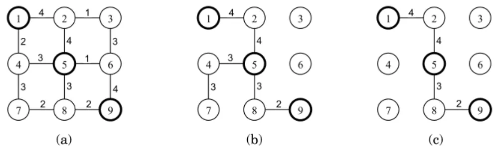
Example 1: Given an instance of rectilinear graph where vertices 1, 5 and 9 are

1 2 3

4 5 6

7 8 9

4 4

4 1

1 3

3 3 2

3

2 2

1 2 3

4 5 6

7 8 9

4 4

3 3 3

2

1 2 3

4 5 6

7 8 9

4 4

3 2

(a) (b) (c)

Figure 2: Illustration of the algorithm (A1)

At the beginning, we label only vertex 1. Then, following edges are added iteratively according to algorithm A1: (1,2), (2,4), (4,5), (4,7), (5, 8), (8,9). Now all terminal vertices are in the tree (Figure 2(b)). We can freely remove vertices 7 and 4 from the Steiner tree because they don't influence the solution. The capacity of the Steiner tree is 2 (Figure 2(c)).

3. MULTICRITERIA STEINER TREE PROBLEM

Given an undirected weighted simple graph G=(N L C Q, , , ) where N, L, C and Q are described in the previous section, we define the bicriterion Steiner tree problem

as a task of finding a Steiner tree with maximal capacity and minimal length. In many cases the process of finding Steiner tree with maximal capacity may give multiple solutions. Under the circumstances it seems appropriate to use the lexicographic method which provides finding the minimal length while keeping the optimal capacity of the tree. The logic inflicts an idea for more precise formulation of the bicriterion Steiner tree problem as a lexicographic optimization problem. It means that the bottleneck Steiner tree problem should be solved first. The optimal solution will determine the maximal capacity of the tree. After that, the next optimization problem to be solved will be classical minisum Steiner tree problem but under the constraint on the capacity of the tree.

Based on the previous considerations the following algorithm for solving the bicriterion Steiner tree problem is proposed:

Algorithm (A2)

1. Solve the bottleneck Steiner tree problem with the algorithm (A1) and find out the maximal capacity M of the tree.

2. Remove from the initial graph all edges with capacity less than M.

3. "Cut the tails" from the graph as mentioned in step 3 of the heuristic (H1) and step 5 of the algorithm (A1). (Those edges certainly will not influence the solution and this will simplify the next step.)

4.

The complexity of Algorithm A2 depends on step 4, i.e. if we chose a heuristic, the algorithm may remain polynomial, but if an exact algorithm is chosen, the whole Algorithm A2 becomes exponential. However, even in case we chose an exact algorithm, the reduction of edges performed in steps 2 and 3 decreases the graph dimension and consequently may significantly decrease the complexity of the whole algorithm.

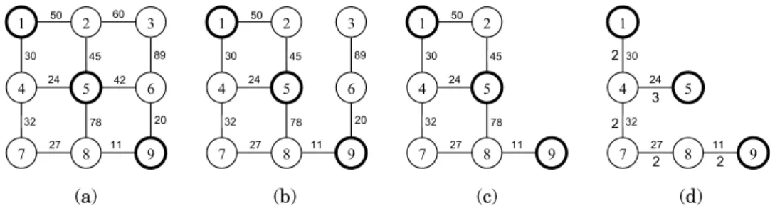
Example 2: For the same instance as in Example 1, the lengths are assigned to each

edge (Figure 3(a)).

1 2 3

4 5 6

7 8 9

50 60

30 45 89

20 78 32

24 42

27 11

1 2 3

4 5 6

7 8 9

50

30 45 89

20 78 32

24

27 11

1 2

4 5

7 8 9

50

30 45

78 32

24

27 11

1

4 5

7 8 9

30

32 24

27 11

2

2 3

2 2

(a) (b) (c) (d)

Figure 3: Illustration of the algorithm (A2)

First we remove all edges that have capacity less than 2 (see the previous example) (Figure 2(b)). After the "cutting" of vertices 3 and 6 the graph in Figure 3(c) will remain. After solving classical STP, final solution is shown in Figure 3(d). This Steiner tree keeps the optimal capacity 2 and under that constraint has a minimal length 124.

It is interesting to notice the following variations of the presented bicriterion Steiner tree problem:

• The same formulation can also be applied to another bicriterion Steiner tree problem where the capacity remains the first criterion while the second one is defined by the number of edges in the tree (which should be minimized). That is a special case of the previous formulation where all edge lengths have the same value (e.g. c_ij=1). Therefore, the same algorithm (A2) can be used for this problem, too.

• The relaxed lexicographic method which allows trading between multiple criteria can also be applied. By introducing parameter α given by the decision maker and by changing step 2 of Algorithm (A2) where only edges with capacity less then M−α should be removed, one can improve the length of

4. NUMERICAL EXPERIENCES

For the purpose of making numerical experiments, the computer program that implements the algorithm (A2) has been developed. As it has been mentioned, the first step of the procedure was implemented through the algorithm (A1). The step 4 of algorithm (A2) is performed by heuristic (H1). As a consequence, the whole procedure has a polynomial complexity. Therefore, no further code optimizations were done.

Hence the second problem (classical Steiner tree problem) remains NP hard, it was interesting to empirically research the level of graph reduction after Step 3 of algorithm (A2). Three parameters were observed: (a) level of vertices reduction

( )

−_{= −1} n1₁₀₀

n

N % where n is a vertices number of starting graph and n is vertices

number after reduction, (b) level of edges reduction

1

( )

−_{= −1} m1₁₀₀

m

M % where m is an

edges number of starting graph and is edges number of remaining graph and (c) maximal capacity M of Steiner tree. All results were obtained as the average of 50

solved instances.

1

m

Instances were generated randomly. For that purpose, two random parameters were used: (a) graph density parameter p which presents probability that edge { ,

exists and (b) range of probably chosen edge capacities R (i.e.

}

i j

rand ( , )

= 1

ij

q R ).

Table 1.

, , :

n t R n=10,t=3,R=4 n=10,t=3,R=4000

p _N− _M− _{M N}− _M− _M

0.1 35 37.9 1.52 39.4 46.0 907 0.3 32 46.5 2.34 41.0 59.0 1580 0.5 20 50.2 2.76 37.2 71.8 2413 0.7 25 67 3.46 31.6 74.2 2709 0.9 22 70.7 3.66 32.8 81.2 3057

, , :

n t R n=100,t=10,R=4 n=100,t=10,R=4000

p _N− _M− _{M N}− _M− _M

0.1 9.4 55.7 3.16 27.1 74.4 2827 0.3 0.5 75.2 4.0 23.0 90.6 3580 0.5 0 75.0 4.0 19.7 93.9 3732 0.7 0 74.9 4.0 24.0 96.0 3818 0.9 0 74.9 4.0 27.3 97.2 3871

, , :

n t R n=316,t=17,R=4 n=316,t=17,R=4000

p _N− _M− _{M N}− _M− _M

Different instances were generated varying 4 parameters: N − number of

vertices, p − graph density, R− range of edge capacities and T− number of terminal

vertices. Experiments have been done with the following values: n∈{10 100 316, , },

{ . , . , . , . , . }, { , , }

∈ 0 1 0 3 0 5 0 7 0 9 ∈ 4 40 4000

p R and t∈ 

{

}

results are presented in Tables 1-3.

In the first set of experiments p and N were varied for all planned values.

Values for R were 4 and 4000 and T was  n. The results are presented in Table 1.

The first thing that can be concluded is that ST capacity is related to both size and density of the graph. As they grow, the capacity gets better and consequently the graph reduction increases. Secondly, smaller instances have greater vertices reduction then the bigger ones, but reduction of edges dramatically increases with the graph dimension. It is interesting to notice that edges reduction was ''stacked'' on one quarter of initial edges number for instances with R=4 (which is the consequence of the uniform distribution of edge capacities) and is much better for instances with

=4000

R . It directly depends on the ST capacity.

That observation initiated new set of experiments with value of R between

these ''extreme'' ones. We chose R=40. Next we wanted to determine how the number of terminal vertices influence graph reduction. The results of these experiments are given in the Table 2.

Table 2.

, , :

n t R n=10,t=3,R=40 n=10,t=5,R=4000

p _N− _M− _{M N}− _M− _M

0.1 43.0 49.9 9.9 25.6 31.9 759 0.3 33.8 46.2 14.4 19.4 40.0 1410 0.5 34.2 69.2 24.8 17.0 54.2 2134 0.7 29.8 75.0 28.9 17.0 68.0 2700 0.9 33.8 82.1 32.8 19.0 77.9 3019

, , :

n t R n=100,t=10,R=40 n=100,t=50,R=4000

p _N− _M− _{M N}− _M− _M

0.1 21.5 70.0 27.8 3.9 55.6 2197 0.3 16.7 88.7 36.2 5.2 85.3 3396 0.5 15.4 93.1 38.1 3.8 91.2 3641 0.7 11.2 94.5 38.7 3.9 93.6 3743 0.9 10.6 95.4 39.1 4.9 95.4 3815

, , :

n t R n=316,t=17,R=40 n=316,t=158,R=4000

p _N− _M− _{M N}− _M− _M

For instances where R=40 the vertices reduction stayed between the values it had in previous instances. ST capacity reached its maximal value (for

) and therefore the number of edges was reduced to

,

=316 =0 7

n p . ₄₀1 of its initial

number. Unlike the instances with R=4 where the maximum was reached with and small density, here the maximum was reached with

=100

n n=316 and greater

density.

Concerning the number of terminal vertices, the conclusion is that its influence on graph reduction is not too big, especially to edges number.

At last, we wanted to check all these trends on greater instances. We tried with , but only 5 instances per result were made (because of time consumption). The results are presented in Table 3. In addition, here we present average values for and m which are described above.

=1000

n

,

1

n m1

Table 3.

, , :

n t R n=1000,t=31,R=4000

p n1 _N− m1 m _N− M

0.1 891.6 21.9 2168 49988 95.7 3823 0.3 928.2 8.2 2307 149806 98.5 3937 0.5 893.4 10.7 1938 249569 99.2 3968 0.7 893.8 10.7 1854 349672 99.5 3979 0.9 814.0 18.6 1622 449502 99.6 3985

It is obvious that the ST capacity increases with the graph size in both number of vertices and number of edges. Column of Table 3 clearly shows the decreasing number of remaining edges although the number of edges in initial graph (column m

Table 3) grows.

1

m

The conclusion is that graph reduction grows proportionally to graph size, but the level of reduction stays polynomial. On the other hand, the complexity of classical Steiner tree problem is NP, so the whole problem remains NP hard. Nevertheless, the graph reduction can move the border of solvable graph size further.

REFERENCES

[1] Climaco, J., and Martins, E.Q.V., "A bicriterion shortest path algorithm", European Journal

of Operational Research, 11 (1982) 399−404.

[2] Cook, W., Cunningham, W., Pulleyblank, W., and Schrijver, A., Combinatorial Optimization,

Series in Discrete Mathematics and Optimization, Wiley-Interscience, 1998.

[3] Cvetkovi}, D., Kova~evi}-Vuj~i}, V., (eds.), Combinatorial Optimization − Mathematical theory

and algorithms, Yugoslav Operational Research Society, Belgrade, 1996. (in Serbian)

[4] Ehtgott, M., Multicriteria Optimization, Springer-Verlag, 2000.

[6] Harris Jr., F.C., "Steiner minimal trees: An introduction, parallel computation and future work", in: D.-Z. Du, P. M. Pardalos (eds.), Handbook of Combinatorial Optimization, Kluwer

Academic Publishers, 1998.

[7] Ivanov, A.O., and Tuzhelin, A.A., Minimal Networks: The Steiner Problem and Its

Generalizations, CRC Press, 1994.

[8] Ulungu, E.L., and Teghem, J., "Multi-objective combinatorial optimization problems: A survey", Journal of Multi-Criteria Decision Analysis, 3 (1994) 83−104.

[9] Vujo{evi}, M., and Stanojevi}, M., "Bottleneck Steiner tree problem", EURO XVII, 17th

European Conference on Operational Research, Budapest, July 16−19, 2000.

[10] Vujo{evi}, M., and Stanojevi}, M., "Multiobjective travelling salesman problem and a fuzzy set

approach to solving it", Application of Mathematics in Engineering and Economics, 27 (2002)

111−118.

[11] Warme, D.M., Winter, P., and Zachariasen, M., "Exact algorithm for plane Steiner tree

problems: A computational study", in: D.-Z. Du, M. Smith, J. H. Rubinstein (eds.), Advances

in Steiner Trees, Kluwer Academic Publishers, 1998.