www.biogeosciences.net/9/4169/2012/ doi:10.5194/bg-9-4169-2012
© Author(s) 2012. CC Attribution 3.0 License.
Biogeosciences
N
2
O emissions from the global agricultural nitrogen cycle – current
state and future scenarios
B. L. Bodirsky, A. Popp, I. Weindl, J. P. Dietrich, S. Rolinski, L. Scheiffele, C. Schmitz, and H. Lotze-Campen
Potsdam Institute for Climate Impact Research (PIK), P.O. Box 60 12 03, 14412 Potsdam, Germany
Correspondence to: B. L. Bodirsky (bodirsky@pik-potsdam.de)
Received: 6 February 2012 – Published in Biogeosciences Discuss.: 13 March 2012 Revised: 19 September 2012 – Accepted: 20 September 2012 – Published: 31 October 2012
Abstract. Reactive nitrogen (Nr) is not only an important
nu-trient for plant growth, thereby safeguarding human alimen-tation, but it also heavily disturbs natural systems. To miti-gate air, land, aquatic, and atmospheric pollution caused by the excessive availability of Nr, it is crucial to understand the
long-term development of the global agricultural Nrcycle.
For our analysis, we combine a material flow model with a land-use optimization model. In a first step we estimate the state of the Nrcycle in 1995. In a second step we create four
scenarios for the 21st century in line with the SRES story-lines.
Our results indicate that in 1995 only half of the Nrapplied
to croplands was incorporated into plant biomass. Moreover, less than 10 per cent of all Nrin cropland plant biomass and
grazed pasture was consumed by humans. In our scenarios a strong surge of the Nrcycle occurs in the first half of the 21st
century, even in the environmentally oriented scenarios. Ni-trous oxide (N2O) emissions rise from 3 Tg N2O-N in 1995
to 7–9 in 2045 and 5–12 Tg in 2095. Reinforced Nrpollution
mitigation efforts are therefore required.
1 Introduction
More than half of the reactive nitrogen (Nr) fixed every year
is driven by human activity (Boyer et al., 2004). The main driver of the nitrogen cycle remains agricultural production, whose ongoing growth will require ever larger amounts of Nr
to provide sufficient nutrients for plant and livestock produc-tion in the future.
The industrial fixation of the once scarce nutrient con-tributed to an unrivaled green revolution of production in the second half of the 20th century. Yet, only 35 to 65 %
of the Nrapplied to global croplands is taken up by plants
(Smil, 1999). The remaining share may interfere with nat-ural systems: The affluent availability of Nr leads to
biodi-versity losses and to the destruction of balanced ecosystems (Vitousek et al., 1997). In the form of nitrous oxide (N2O),
Nrcontributes to global warming (Forster et al., 2007) and is
the single most important ozone depleting substance (Ravis-hankara et al., 2009). Finally, it contributes to soil (Velthof et al., 2011), water (Grizzetti et al., 2011), and air pollution (Moldanova et al., 2011). Brink et al. (2011) estimate that the damage caused by nitrogen pollution adds up to 70–320 billion Euro in Europe alone, equivalent to 1–4 % of total in-come.
Therefore, much effort has been dedicated to improving our knowledge about the global agricultural Nrcycle. Smil
(1999) pioneered the creation of the first comprehensive global Nrbudget, and determined the key Nrflows in
agricul-ture, most importantly fertilizer application, biological nitro-gen fixation, manure application, crop residue management, leaching, and volatilisation. Sheldrick et al. (2002) extended the nutrient budgets to phosphorus and potash. Galloway et al. (2004) included natural terrestrial and aquatic systems in the Nrcycle. Liu et al. (2010a) broke up the global
agricul-tural nutrient flows to a spatially explicit level. Bouwman et al. (2005, 2009, 2011) were the first, and so far the only, to have simulated the future development of the Nrcycle with
detailed regional Nrflows.
However, the description of the current state of the Nr
cy-cle was often incomprehensive. Belowground residues were so far not considered explicitly by other global studies, even though they withdraw large amounts of Nr from soils, and
their decay on fields contributes to Nrlosses and emissions.
budgets, although they make up a considerable share of total cropland production. Furthermore, no bottom-up estimate for Nrrelease by the loss of soil organic matter exists so far.
Re-garding future projections, substitution effects between dif-ferent Nrinputs are usually not considered.
In this paper, we create new estimates for the state of the agricultural Nrcycle in 1995 and four future scenarios
un-til 2095 based on the SRES storylines. Our study presents a comprehensive description of the Nrcycle and covers Nr
flows that have not been regarded by other studies so far. We create detailed cropland Nrbudgets, but also track Nrflows
upstream towards the processing sector, the livestock system and final consumption. This unmasks the low Nr efficiency
in agricultural production. We use an independent parametri-sation of the relevant Nr flows, concerning for example Nr
in crop residues or biological Nrfixation. This allows for the
identification of uncertainties in current estimates. For future projections we use a closed budget approach that allows for substitution between cropland Nr inputs (like fertilizer,
ma-nure or crop residues) and for an endogenous calculation of livestock Nrexcretion. The budget approach is also used to
estimate total nitrogen losses from fertilization and manure management (the sum of N2, NOx, NHyand N2O
volatilisa-tion as well as Nrleaching). As N2O emissions play a crucial
role in a global context, our model estimates them explicitly. For this purpose, our study uses the emission parameters of the 2006 IPCC Guidelines for National Greenhouse Gas In-ventories (Eggleston et al., 2006).
The paper is set up as follows: In the methods section, we first describe the Model of Agricultural Production and its Impact on the Environment (MAgPIE) that delivers the framework for our analysis. Then we give an overview on the implementation of crop residues, conversion byproducts and manure in the model. The description of all major Nrflows
is followed by a summary of the scenario designs. In the re-sults section, we present our simulation outputs for the state of the Nrcycle in 1995 and our projections for inorganic
fer-tilizer consumption, N2O emissions and other important Nr
flows. In the discussion section, we compare our estimates to other studies and integrate the findings to a comprehensive cropland Nrbudget for 1995, highlighting the largest
uncer-tainties. We also compare our scenarios for the rise of the Nr
cycle in the 21st century to estimates of other studies. As it is a key driver of the Nrcycle, we examine the livestock sector
in more detail. Finally, the implications of our findings on the threat of Nrpollution are followed by our conclusions and an
outlook on the opportunities for mitigation.
2 Materials and methods
2.1 General model description
MAgPIE (Lotze-Campen et al., 2008; Popp et al., 2010, 2012; Schmitz et al., 2012) is a model well suited to
per-NAM
PAO FSU
CPA SAS MEA EUR
AFR LAM
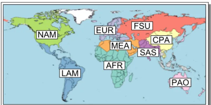
Fig. 1. The ten MAgPIE world regions. Sub-Sahara Africa (AFR),
Centrally Planned Asia (CPA), Europe (including Turkey) (EUR), Former Soviet Union (FSU), Latin America (LAM), Middle East and North Africa (MEA), North America (NAM), Pacific OECD (Australia, Japan and New Zealand) (PAO), Pacific Asia (PAS), and South Asia (SAS).
forming assessments of agriculture on a global scale and to simulating long-term scenarios. It is comprehensive concern-ing the spatial dimension and covers all major crop and live-stock sectors. Moreover, it features the major dynamics of the agricultural sector, like trade, technological progress or land allocation according to the scarcity of suitable soil, wa-ter and financial resources. As it treats agricultural produc-tion not only as economic value but also as physical good, it can easily perform analysis of material flows.
The existing model (as described in the Supplement) has been extended by a number of features in order to describe the dynamics of the Nrcycle. Crop residues and conversion
byproducts from crop processing make up a major share of total biomass and were therefore integrated into the model (Sect. 2.2). Moreover, all dry matter flows were transformed into Nr flows. Nr flows in manure management, cropland
fertilization and the transformation of Nr losses into
emis-sions were included (Sect. 2.3). Finally, the scenario setup is described in Sect. 2.4. Detailed documentation as well as a mathematical description of all model-extensions can be found in Appendix A.
2.2 Crop residues and conversion byproducts
As official global statistics exist only for crop production and not for crop residue production, we obtain the biomass of residues by using crop-type specific plant growth functions based on crop production and area harvested. Plant biomass is divided into three components: the harvested organ as listed in FAO, the aboveground (AG) and the belowground (BG) residues. For AG residues of cereals, leguminous crops, potatoes and grasses, we use linear growth functions (Eggle-ston et al., 2006) with a positive intercept which accounts for the decreasing harvest index with increasing yield. For crops without a good matching to the categories of Eggleston et al. (2006), we use constant harvest indices (Wirsenius, 2000; Lal, 2005; Feller et al., 2007).
Based on Smil (1999), we assume that 15 % of AG crop residues in developed and 25 % in developing regions are burned in the field. Furthermore, developing regions use 10 % of the residues to settle their demand for building ma-terials and household fuel. The demand for crop residues for feed is calculated based on crop residues in regional livestock specific feed baskets from Weindl et al. (2010). The remain-ing residues are assumed to be left on the field. We estimate BG residue production by multiplying total AG biomass (har-vest + residue) with a crop-specific AG to BG ratio (Eggle-ston et al., 2006; Khalid et al., 2000; Mauney et al., 1994). All BG crop residues are assumed to be left on the field.
Conversion byproducts like brans, molasses or oil cakes occur during the processing of crops into refined food. We link the production of conversion byproducts to the domestic supply of the associated crops using a fixed regional conver-sion ratio. Feed demand for converconver-sion byproducts is based on feed baskets from Weindl et al. (2010) and rises with live-stock production in the region. All values are calibrated to meet the production and demand for conversion byproducts of FAO in 1995 (FAOSTAT, 2011). In case the future demand for feed residues or crop byproducts exceeds the production, they can be replaced by feedstock crops of the same nutri-tional value.
2.3 Nrflows
2.3.1 Nrcontent of plant biomass, conversion byproducts and food
The biomass flows of the MAgPIE model are transformed into Nrflows, using product-specific Nr contents. We
com-pile the values for harvested crops, conversion byproducts, AG and BG residues from Wirsenius (2000); Fritsch (2007); FAO (2004); Roy et al. (2006); Eggleston et al. (2006) and Khalid et al. (2000). The Nr in vegetal food supply is
esti-mated by subtracting the Nrin conversion byproducts from
Nrin harvest dedicated for food. Nrin livestock food supply
is calculated by multiplying the regional protein supply from each commodity group of FAOSTAT (2011) with protein to Nrratios of Sosulski and Imafidon (1990) and Heidelbaugh
et al. (1975). As food supply does not account for waste on the household-level, we use regional intake to supply shares from Wirsenius (2000).
2.3.2 Manure management
The quantity of Nrin livestock excreta is calculated
endoge-nously from Nrin feed intake (consisting of feedstock crops,
conversion byproducts, crop residues and pasture) and live-stock productivity. The Nrin feed minus the amount of Nrin
the slaughtered animals, milk and eggs equals the amount of Nrin manure. To estimate the mass of slaughtered animals,
we multiply the FAO meat production with livestock-specific carcass to whole body weight ratios from Wirsenius (2000). Nr contents of slaughtered animals, milk and eggs are
ob-tained from Poulsen and Kristensen (1998).
Manure from grazing animals on pasture is assumed to be returned to pasture soils except a fraction of manure be-ing collected for household fuel in some developbe-ing regions (Eggleston et al., 2006). Manure from feedstock crops and conversion byproducts are assumed to be excreted in ani-mal houses. We estimate that one quarter of the Nrin crop
residues used as feed in developing regions stems from stub-ble grazing on croplands, while the rest is assigned to animal houses. Finally, we distribute all manure in animal houses be-tween 9 different animal waste management systems accord-ing to regional and livestock-type specific shares in Eggle-ston et al. (2006).
2.3.3 Cropland Nrinputs
In our model, cropland Nr inputs include manure, crop
residues left in the field, biological Nr fixation, soil organic
matter loss, atmospheric deposition, seed and inorganic fer-tilizer.
in developed regions. Additionally, all Nr excreted during
stubble grazing is returned to cropland soils.
For crop residues left in the field, we assume that all Nris
recycled to the soils, while 80–90 % of the residues burned in the field are lost in combustion (Eggleston et al., 2006).
Nrfixation by free living bacteria in cropland soils and rice
paddies is taken into account by assuming fixation rates of 5 kg per ha for non-legumes and 33 kg per ha for rice (Smil, 1999). The Nrfixed by leguminous crops and sugar cane is
estimated by multiplying Nrin plant biomass (harvested
or-gan, AG and BG residue) with regional plant-specific per-centages of plant Nr derived from N2 fixation (Herridge et
al., 2008).
Nrrelease by the loss of soil organic matter after the
con-version of pasture land or natural vegetation to cropland is es-timated based on the methodology of Eggleston et al. (2006). Our estimates for 1995 use a dataset of soil carbon under nat-ural vegetation from the LPJmL model (Sitch et al., 2003; Gerten et al., 2004; Bondeau et al., 2007). For 1995, we use historical land expansion from the HYDE-database (Klein Goldewijk et al., 2011a), while the land expansion in the fu-ture is estimated endogenously by MAgPIE.
The regional amount of atmospheric deposition on crop-lands for 1995 is taken from Dentener (2006). For future sce-narios, we assume that the atmospheric deposition per crop-land area grows with the same growth rate as the average regional agricultural NOxand NHyemissions.
The amount of harvest used for seed is obtained from FAOSTAT (2011). We multiply the seed with the Nr share
of the harvested organ to estimate Nrin seed returned to the
field.
Regional inorganic fertilizer consumption in 1995 is ob-tained from IFADATA (2011). For the scenarios, we use a closed budget approach. For this purpose, we define cropland soil Nruptake efficiency (SNUpE) as the share of Nrinputs
to soils (fertilizer, manure, residues, atmospheric deposition, soil organic matter loss and free-living Nrfixers) that is
with-drawn from the soil by the plant. These withdrawals from the soil are calculated by subtracting Nrderived not from the soil
(seed and internal biological fixation by legumes and sugar-cane) from Nr in plant biomass. SNUpE is calculated on a
regional level for the year 1995 and becomes an exogenous scenario parameter for future estimates. Its future develop-ment is determined by the scenario storyline (see Sect. 2.4).
In future scenarios, the soil withdrawals and the exogenous SNUpE determine the requirements for soil Nrinputs. If the
amount of organic fertilizers is not sufficient, the model has to apply as much nitrogen fertilizer as it requires to balance out the budget. In our model, the Nr inputs to crops have
no influence on the yield. We assume in reverse that a given crop yield can only be reached with sufficient Nrinputs. An
eventual Nrlimitation is already reflected in the height of the
crop yield.
2.3.4 Emissions
Emission calculations are in line with the 2006 IPCC Guide-lines of National Greenhouse Gas Emissions (Eggleston et al., 2006), accounting for NOx, NHyas well as direct and
in-direct N2O emissions from managed soils, grazed soils and
animal waste. Our estimates neither cover agricultural N2O
emissions from savannah fires, agricultural waste burning or cultivation of histosols, nor emissions from waste disposal, forestry or fertilizer production. Emission factors are con-nected directly to the corresponding Nr flows of inorganic
fertilizer application, as well as residue burning and decay on field, manure management, manure application, direct ex-cretion during grazing, and soil organic matter loss. We use a Monte Carlo analysis to estimate the effect of the uncertainty of the IPCC emission parameters on global N2O emissions. 2.4 Future scenarios
For future projections, we analyse four scenarios based on the SRES storylines (Nakicenovic et al., 2000), varying in two dimensions: economy versus ecology and globalisation versus heterogeneous development of the world regions. The parametrisation of these scenarios differs in several aspects, which try to cover the largest uncertainties for the future de-velopment of the Nr cycle (Table 1). In the following, the
scenario settings are shortly described, while a detailed de-scription and an explanation of the model implementation is provided in Appendix A4.
Food demand projections and the share of calories from livestock products are calculated based on regressions be-tween income and per-capita calorie demand (intake and household waste), as well as regressions between income and the share of livestock calories in total demand. The regres-sions are based on a panel dataset (5889 data points) from FAOSTAT (2011) and WORLDBANK (2011) for 162 coun-tries from 1961 to 2007. In the environmentally oriented sce-narios, we used different functional forms for the regressions that result in lower values for plant and livestock demand. The future projections are driven by population and GDP sce-narios from the SRES marker scesce-narios (CIESIN, 2002a,b).
Trade in MAgPIE is oriented along historical trade pat-terns, fixing the share of products a region has imported or exported in the year 1995. To account for trade liberalisa-tion, an increasing share of products can be traded according to comparative advantages in production costs instead of his-torical patterns. We use two different trade scenarios based on Schmitz et al. (2012), assuming faster trade liberalisation in the globalised scenarios.
Table 1. Scenario definitions, based on the IPCC SRES scenarios.
1995 2045 2095
A1 A2 B1 B2 A1 A2 B1 B2
GDP (1012US$) 34 222 106 170 138 674 314 453 319
Population (109heads) 5.7 8.6 10.8 8.6 9.2 7.4 14.8 7.4 10.4
Food demand (1018J) 23 46 50 42 43 47 81 41 53
– Thereof livestock products 16 % 24 % 17 % 22 % 22 % 22 % 17 % 16 % 18 %
Trade patterns
– Historical 100 % 60 % 88 % 60 % 88 % 37 % 78 % 37 % 78 %
– Comparative advantage 0 % 40 % 12 % 40 % 12 % 65 % 22 % 65 % 22 %
Livestock systems
– Current mix 100 % 20 % 50 % 20 % 50 % 0 % 20 % 0 % 20 %
– Industrialised 0 % 80 % 50 % 80 % 50 % 100 % 80 % 100 % 80 %
Animal waste1
– Current mix 100 % 30 % 80 % 40 % 80 % 0 % 50 % 20 % 50 %
– Daily spread 0 % 0 % 0 % 30 % 20 % 0 % 0 % 40 % 50 %
– Anaerobic digester 0 % 70 % 20 % 30 % 0 % 100 % 50 % 40 % 0 %
Soil Nruptake efficiency (SNUpE) 51 %2 60 % 55 % 65 % 65 % 60 % 60 % 70 % 70 %
Intact and frontier forest protection no no yes yes no no yes yes
1Only for waste in animal houses. 2Global average.
productive system has a large proportion of feedstock crops and conversion byproducts in the feed baskets. In the glob-alised scenarios, convergence is assumed to be faster than in the regionalised scenarios.
Currently, regional animal waste management systems are diverse and their future development is highly uncertain. We assume two major future trends. Firstly, due to the scarcity of fossil fuels and the transformation of the energy system towards renewables, the use of animal manure as fuel for bioenergy will become increasingly important. Secondly, in the environmental scenarios, we also assume that an increas-ing share of manure is spread to soils in a timely manner. We therefore shift the current mix of animal waste man-agement systems gradually towards anaerobic digesters and daily spread.
Improvements in the cropland soil Nr uptake efficiency
may occur in the future due to increasing environmental awareness or to save input costs. The regional efficiencies have been calculated for 1995, and we assume that they grad-ually increase in all scenarios, with the environmental scenar-ios reaching the highest efficiencies.
Finally, the expansion of agricultural area into unpro-tected intact and frontier forests is restricted gradually until 2045 in the environmental oriented scenarios, as described in Schmitz (2012).
The scenarios start in the calibration year 1995 and con-tinue until 2095. The base year 1995 facilitates the compar-ison with other studies (Smil, 1999; Sheldrick et al., 2002; Liu et al., 2010a) and allows for a consistency check and benchmarking between the scenarios and the real develop-ment since 1995.
3 Results
Detailed global and regional results of the current state of the agricultural Nrcycle and the four scenarios can be found in
the Supplement. In the following, the most important results are summarised.
3.1 Global nitrogen cycle
3.1.1 State in 1995
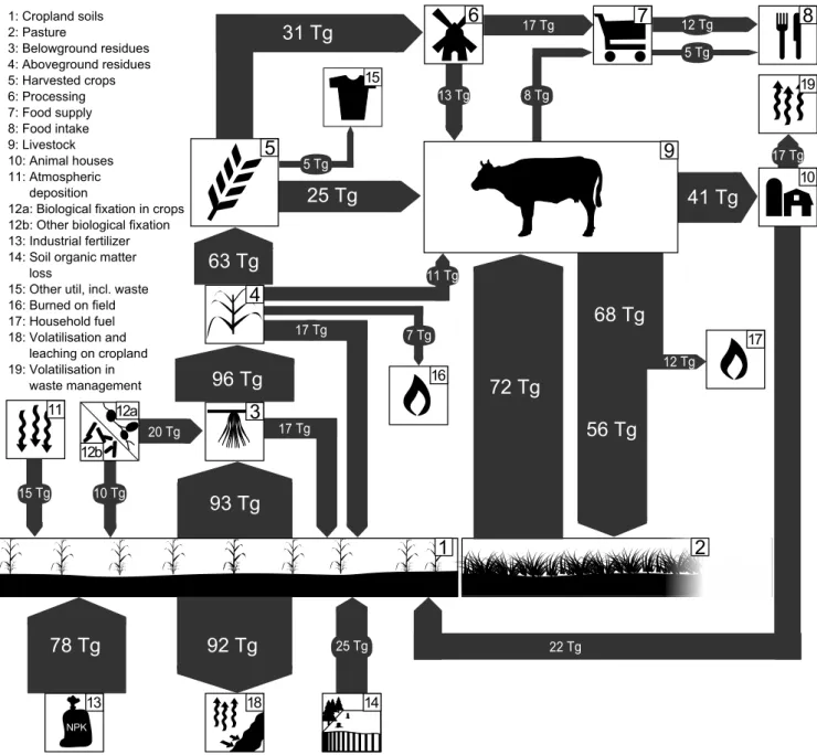
According to our calculations for the year 1995, 205 Tg Nr
are applied to or fixed on global cropland, of which 115 is taken up by cropland plant biomass. Thereof, 50 Tg are fed to animals in the form of feedstock crops, crop residues, or conversion byproducts, plus an additional 72 Tg from grazed pasture, to produce animal products which contain 8 Tg Nr.
In total, plant and animal food at whole market level contains 24 Tg Nr, of which finally only 17 Tg Nrare consumed.
Fig-ure 2 shows an in-depth analysis of Nr flows in 1995 on a
global level.
3.1.2 Scenarios
In our four scenarios, the throughput of the Nr cycle rises
considerably within the 21st century. Total Nr in cropland
plant biomass reaches 244 (B2)–323 (A1) Tg Nrin 2045 and
251 (B1)–434 (A2) Tg Nrin 2095. Also, the range of soil
in-puts increases throughout the century, starting with 185 Tg in 1995 to 286 (B2)–412 (A1) Tg Nrin 2045 and 286 (B1)–
553 (A2) Tg Nrin 2095. Inorganic fertilizer consumption in
17 Tg
1
2
3
4
5
6
7
8
9
11 12a
12b
NPK
13 14
15
16
17
18
10 19
1: Cropland soils 2: Pasture
3: Belowground residues 4: Aboveground residues 5: Harvested crops 6: Processing 7: Food supply 8: Food intake 9: Livestock 10: Animal houses 11: Atmospheric deposition
12a: Biological fixation in crops 12b: Other biological fixation 13: Industrial fertilizer 14: Soil organic matter loss
15: Other util, incl. waste 16: Burned on field 17: Household fuel 18: Volatilisation and leaching on cropland 19: Volatilisation in
waste management
72 Tg
41 Tg
68 Tg
56 Tg
93 Tg
96 Tg
63 Tg
31 Tg
92 Tg
78 Tg
25 Tg
12 Tg
15 Tg 10 Tg
5 Tg 12 Tg
7 Tg
25 Tg
20 Tg 17 Tg
5 Tg
8 Tg 13 Tg
17 Tg
11 Tg
22 Tg 17 Tg
Fig. 2. Agricultural Nrcycle in Tg Nrin the year 1995. Flows below 5 Tg Nrare not depicted. No estimates were made for Nrinputs to pasture soils by atmospheric deposition and biological fixation.
(A1) Tg Nruntil 2045 and a stagnating or even declining
con-sumption thereafter, while the A scenarios exhibit a much stronger and continuous increase to 173 (A1) and 177 (A2) Tg Nr in 2045, and 214 (A1) and 260 (A2) Tg Nr in 2095
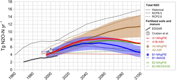
(Fig. 3). Despite these wide ranges, the differences of N2O
emissions between the scenarios is in the first half of the cen-tury rather narrow. They start with 3.9 Tg N2O-N in 1995,
with a range of 3.0 to 4.9 Tg N2O-N being the 90 %
con-fidence interval for uncertainty of the underlying emission parameters of Eggleston et al. (2006). Up to 2045, they rise to 7.2 (5.4 to 9.0) Tg N2O-N in the B1 scenario and 8.6 (6.6
to 10.5) Tg N2O-N in the A2 scenario, and widen towards
the end of the century to 4.9 (3.5 to 6.4) Tg N2O-N in the B1
scenario and 11.6 (8.8 to 14.2) Tg N2O-N in the A2 scenario
(Fig. 4).
3.2 Regional budgets
While the surge of the Nrcycle can be observed in all regions,
the speed and characteristics are very different between re-gions (Table 2). Sub-Saharan Africa (AFR), South Asia (SAS), and Australia and Japan (PAO) show the strongest rel-ative increases in harvested Nr, while in Europe (EUR) and
Table 2. Regional estimates of Nrflows for the state in 1995 and for the four scenarios A1A2||BB21in Tg Nrper year. Losses consist of losses from cropland soils and animal waste management.
Nrflow Year World Regions
AFR CPA EUR FSU LAM MEA NAM PAO PAS SAS
Harvest 1995 63 3 12 10 5 6 2 13 2 3 7
2045 182 160 15 14 30 28 15 14 10 9 29 21 10 10 20 19 17 11 6 5 30 29
153 143 12 12 26 28 15 14 9 9 22 19 8 7 23 20 10 7 6 5 21 22
2095 196 137 20 9 33 27 16 13 11 8 26 13 14 12 21 17 18 7 5 3 33 29
260 169 24 19 38 30 19 15 13 11 50 22 13 9 32 21 25 9 10 6 35 29
Residues 1995 35 3 6 4 3 4 1 6 1 2 5
2045 94 85 10 9 15 15 7 7 7 7 16 13 4 4 10 9 9 6 4 4 12 12
73 67 8 7 12 13 6 6 4 4 11 9 3 2 10 8 5 3 4 3 11 10
2095 98 76 11 7 17 15 7 6 8 7 15 9 5 5 11 9 8 3 4 3 13 12
114 76 12 10 19 14 8 6 5 4 21 9 5 3 13 9 11 4 6 3 15 12
Fertilizer 1995 78 1 24 13 2 4 3 13 1 4 13
2045 173 145 9 7 40 36 13 13 11 9 6 7 15 14 23 21 33 19 5 3 20 15
177 122 14 8 41 30 21 16 8 5 7 10 11 8 30 20 18 9 6 4 22 11
2095 214 128 0 0 50 39 21 16 12 8 23 0 23 17 19 15 32 12 4 4 24 17
260 131 19 10 59 35 22 15 10 7 20 5 12 9 37 20 46 12 7 5 27 12
Manure 1995 111 15 12 13 7 21 3 10 4 3 22
2045 241 217 65 60 28 22 20 15 8 7 63 55 7 7 9 6 3 2 6 5 32 39
250 262 51 56 26 37 17 13 10 9 58 52 11 8 14 9 5 3 9 9 49 65
2095 205 131 105 44 16 12 6 2 7 5 23 36 5 3 17 8 2 1 4 2 19 18
332 240 69 69 34 26 21 10 11 5 92 51 20 11 17 5 5 1 12 7 50 55
Biol. Nr 1995 27 2 4 2 2 4 0 5 1 2 4
2045 72 61 8 7 8 7 5 4 4 4 17 11 1 1 8 7 2 2 4 2 17 16
57 56 6 6 6 8 4 3 4 4 13 11 1 1 8 8 2 2 3 2 10 11
2095 75 46 11 4 9 5 4 3 5 3 15 6 1 1 7 6 3 0 1 1 20 17
95 64 12 8 7 7 4 4 5 6 30 12 3 2 11 8 3 2 4 2 17 14
Trade 1995 0 0 -1 -2 -1 2 -2 4 0 -1 0
2045 0 0 -8 -8 -1 3 -6 -3 1 1 -11 -14 -2 -1 10 11 14 8 -3 -2 9 6
0 0 -3 -6 -4 -7 -1 1 1 2 1 3 -7 -4 10 11 7 4 -4 -4 1 0
2095 0 0 -51 -21 16 14 6 7 1 0 4 -21 0 1 0 6 14 5 -3 -3 14 11
0 0 -5 -15 -6 1 -2 4 1 6 -3 -8 -19 -6 15 14 20 8 -6 -3 4 -2
Losses 1995 109 5 27 15 9 8 3 18 3 7 15
2045 180 146 17 16 32 27 15 13 11 10 28 23 10 9 18 14 19 10 7 6 21 19
201 137 18 14 37 31 21 14 11 8 27 16 10 7 27 16 13 6 10 7 25 18
2095 197 103 39 11 31 20 14 8 12 7 23 14 14 8 19 11 18 5 6 3 21 15
257 131 25 19 45 25 21 11 12 6 43 19 14 8 30 12 26 6 12 5 29 19
N2O 1995 3.9 0.4 0.7 0.5 0.3 0.7 0.1 0.6 0.1 0.2 0.4
2045 8.1 7.2 1.4 1.3 1.1 1 0.6 0.5 0.4 0.3 1.8 1.6 0.4 0.4 0.6 0.5 0.6 0.4 0.3 0.2 0.9 0.9
8.6 7.5 1.3 1.3 1.2 1.3 0.7 0.5 0.4 0.3 2 1.6 0.4 0.3 0.9 0.6 0.4 0.2 0.3 0.3 1 1
2095 7.2 4.9 1.8 0.8 1 0.8 0.5 0.3 0.4 0.3 0.8 0.8 0.5 0.4 0.7 0.5 0.6 0.2 0.2 0.1 0.7 0.6
increase in production in AFR is not sufficient to settle do-mestic demand, such that large amounts of Nrhave to be
im-ported from other regions. Also the Middle East and North-ern Africa (MEA) have to import large amounts of Nr due
to the unsuitable production conditions and high population growth. At the same time, AFR requires only low amounts of inorganic fertilizer, as the domestic livestock production fed with imported Nrprovides sufficient nutrients for production.
In the globalised scenarios A1 and B1, the overspill of ma-nure even reduces the actual soil nutrient uptake efficiency (SNUpE) in 2095 with 0.41 (A1) and 0.67 (B1), below the potential scenario value of 0.6 or 0.7.
Despite its large increase in consumption, SAS does not require large imports, as it can also settle its Nr
require-ments with a balanced mix of biological fixation, manure, crop residues and inorganic fertilizer. Similarly, Latin Amer-ica can cover large parts of its Nr demand with
biologi-cal fixation and manure. In comparison with this, the large exporters North America (NAM) and Pacific OECD (PAO) have a much stronger focus on fertilization with inorganic fertilizers.
In the globalised scenarios, these characteristics tend to be more pronounced than in the regionalised scenarios, as each region specialises in its relative advantages. The structural differences between the economical and ecological oriented scenarios are less distinct, yet it can be observed that the re-duced livestock consumption in developed regions leads to a lower importance of manure and a generally lower harvest of Nrin these regions.
4 Discussion
This study aims to create new estimates for the current state and the future development of the agricultural Nrcycle. For
this purpose, we adapted the land-use model MAgPIE to cal-culate major agricultural Nr flows. As will be discussed in
the following, the current size of the Nrcycle is much higher
than previously estimated. The future development of the Nr
cycle depends largely on the scenario assumptions, which we based on the SRES storylines (Nakicenovic et al., 2000). We expect the future rise of the Nrcycle to be higher than
sug-gested by most other studies. Thereby, the livestock sector dominates both the current state and future developments. The surge of the Nr cycle will most likely be accompanied
by higher Nrpollution.
4.1 The current state of the agricultural Nrcycle
Data availability for Nr flows is poor. Beside the
consump-tion of inorganic fertilizer, no Nr flow occurs in official
statistics. Even the underlying material flows, like produc-tion and use of crop residues or animal manure are usually not recorded in international statistics. Therefore, indepen-dent model assessments are required, using different
method-ologies and parametrisations to identify major uncertainties. In the following we compare our results mainly with esti-mates of Smil (1999), Sheldrick et al. (2002) and Liu et al. (2010a), as summarised in Table 3.
The estimates for Nr withdrawals by crops and
above-ground residues are relatively certain. They have now been estimated by several studies using different parametrisations. The scope between the studies is still large with 50 to 63 Tg Nrfor harvested crops and 25 to 38 Tg Nrfor residues,
whereby the estimate of Sheldrick et al. (2002) may be too high due to the missing correction for dry matter when esti-mating nitrogen contents (Liu et al., 2010b).
Large uncertainties can be attributed to the cultivation of fodder and cover crops. They represent a substantial share of total agricultural biomass production, and they are rich in Nrand often Nrfixers. Yet, the production area, the species
composition and the production quantity are highly uncer-tain, and no reliable global statistics exist. The estimate from FAOSTAT (2005) used by our study has been withdrawn without replacement in newer FAOSTAT releases. It counts 2900 Tg fresh matter fodder production on 190 million ha (Mha). Smil (1999) appraises the statistical yearbooks of 20 large countries and provides a lower estimate of only 2500 Tg that are produced on 100–120 Mha.
Estimates for Nr in animal excreta diverge largely in the
literature. Using bottom-up approaches based on typical ex-cretion rates and Nrcontent of manure, Mosier et al. (1998)
and Bouwman et al. (2011) calculate total excretion to be above 100 Tg Nr. Smil (1999) assumes total excretion to be
significantly lower with only 75 Tg Nr. Our top-down
ap-proach, using the fairly reliable feed data of the FAOSTAT database, can support the higher estimates of Mosier et al. (1998) and Bouwman et al. (2011), with an estimate of 111 Tg Nr. The same global total of 111 Tg Nr can be
ob-tained bottom-up if one multiplies typical animal excretion rates taken from Eggleston et al. (2006) with the number of living animals (FAOSTAT, 2011). Yet, regional excretion rates diverge significantly; the top-down approach leads to considerably higher rates in Africa and the Middle East and lower rates in South and Pacific Asia.
Biological Nrfixation is another flow of high uncertainty
and most studies still use the per ha fixation rates of Smil (1999) for legumes, sugarcane and free-living bacteria. Cur-rently no better estimate exists for free-living bacteria (Her-ridge et al., 2008). However, they contribute only a minor in-put to the overall Nrbudget with little impacts on our model
results. To estimate the fixation by legumes and sugarcane, we use a new approach based on percentages of plant Nr
de-rived from fixation, similar to Herridge et al. (2008). This, in combination with total above- and belowground Nr
con-tent of a plant, can predict Nrfixation more accurately.
How-ever, the parametrisation of Herridge et al. (2008) probably overestimates Nrfixation, especially for soybeans. Most
im-portantly, the Nrcontent of the belowground residues as well
with Eggleston et al. (2006), Sivakumar et al. (1977) or Do-gan et al. (2011). Also the Nrcontent of the shoot seems too
high given that soybean residues have a much lower Nr
con-tent than the beans (Fritsch, 2007; Wirsenius, 2000; Eggle-ston et al., 2006). Correcting the estimates of Herridge et al. (2008) for the water content of the harvested crops further re-duces their estimate. If one finally accounts for the difference in base year between the two estimates, with global soybean production increasing by 69 % between 1995 and 2005, we come to a global total fixation from legumes and sugarcane of 9 Tg Nrin 1995 as opposed to 21 Tg Nrin 2005 in the case
of Herridge et al. (2008). Our estimate is in between the esti-mates of Smil (1999) and Sheldrick et al. (2002), even though we used a different approach.
Accumulation or depletion of Nr in soils has so far been
neglected in future scenarios (Bouwman et al., 2009, 2011), assuming that soil organic matter is stable and all excessive Nr will volatilise or leach. However, the assumption of a
steady state for soil organic matter should not be valid for land conversion or for the cultivation of histosols. Our rough bottom-up calculations estimate that the depletion of soil organic matter after transformation of natural vegetation or pasture to cropland releases 25 Tg Nrper year. With a yearly
global average release of 122 kg Nrper ha newly converted
cropland, the amount of Nr released may exceed the
nutri-ents actually required by the crops, especially in temperate, carbon rich soils. Vitousek et al. (1997) estimates that the cultivation of histosols and the drainage of wetlands releases another 10 Tg Nrper year, although it is unclear how much
thereof enters agricultural systems.
The total size of the cropland Nrbudget is larger than
es-timated by previous studies. This can be attributed less to a correction of previous estimates than to the fact that past studies did not cover all relevant flows. In Table 3 we sum-marise cropland input and withdrawals mentioned by previ-ous studies. The sum of all withdrawals (Total OUT) ranges between 81 and 115 Tg Nr. However, if the unconsidered
flows are filled with estimates from other studies, the cor-rected withdrawals (Total OUT∗) shifts to 105–134 Tg Nr.
The same applies to inputs, where the range shifts and nar-rows down from 137–205 Tg Nr total inputs (Total IN) to
198–232 Tg Nrtotal inputs when all data gaps are filled
(To-tal IN∗). The Nr uptake efficiency (NUpE∗), defined as the
fraction of IN∗ which is incorporated into OUT∗ remains within the plausible global range of 0.35–0.65 defined by Smil (1999) for all studies. In our study, this holds even for every MAgPIE world region. SNUpE and SNUpE∗ are slightly higher, with 49 % and 51 % of Nrapplied to soils
be-ing taken up by the roots of crops. The corrected estimates for total losses (Losses∗) is, with 84–112 Tg Nr, significantly
higher than previously estimated.
Table 3. Comparison of global cropland soil balances.
This Smil Sheldrick Liu
study (1999b) (1996) (2010)
Base year 1995 1995 1996 2000
OUT
Crops 50 50 63 52
Crop residues 31 25 38 29
Fodder 13 10 – –
Fodder residues 4 – – –
BG residues 17 – – –
IN
Residues 12 14 23 11
Fodder residues 4 – – –
BG residues 17 – – –
Legume fixation 9 10 8
22
Other fixation 10 11 –
Fixation fodder 11 12 – –
Atm. deposition 15 20 22 14
Manure on field 24 18 25 17
Seed 2 2 – –
Irrigation water – 4 – 3
Sewage – – 3 –
Soil organic 25 – – –
matter loss
Fertilizer 78 78 78 68
Histosols – – – –
BALANCE
Total OUT 115 85 101 81
Total OUT∗ 115 105 134 114
Total IN 205 169 159 137
Total IN∗ 212 217 232 198
Losses 91 80 75 67
Losses∗ 98 112 97 84
NUpE 0.56 0.50 0.64 0.59
NUpE∗ 0.54 0.48 0.58 0.58
SNUpE 0.51 0.42 0.62 0.51
SNUpE∗ 0.49 0.42 0.54 0.48
∗Data gaps are filled with estimates from other studies. We use estimates by this study if available; for irrigation we use Smil (1999), for sewage Sheldrick et al. (2002), and for histosols no estimate exists.
4.2 Scenario assumptions
The simulation of the widely used SRES storylines (Nakicen-ovic et al., 2000) facilitates the comparison with other studies like Bouwman et al. (2009) or Erisman et al. (2008) and al-lows for the integration of our results into other assessments. However, the SRES storylines provide only a qualitative de-scription of the future. In the following, the key assumptions underlying our parametrisation and model structure shall be discussed.
dynamics. They merely diverge in the interpretation of past dynamics or the magnitude of change assigned to certain trends. Population grows at least until the mid of the 21st century, and declines first in developed regions. Per-capita income grows throughout the century in all scenarios and all world regions, and developing regions tend to have higher growth rates than developed regions. This has strong impli-cations on the food demand, which is driven by both pop-ulation and income growth. As food demand is a concave function of income, it depends mostly on the income growth in low-income regions. In the first half of the century, the pressure from food demand is therefore highest in the high-income A1 scenario. In the second half, the A2 scenario also reaches a medium income and therefore a relatively high per capita food demand. Additionally, the population growth di-verges between the scenarios in the second half of the cen-tury, with the A2 scenario reaching the highest world pop-ulation and as a consequence the highest food demand. As food demand is exogenous to our model, price effects on con-sumption are not captured by the model. However, even in the A2 scenario the shadow prices (Lagrange multipliers) of our demand constraints increase globally by 0.5 % per year until 2045, with no region showing higher rates than 1.1 %. This indicates only modest price pressure, lagging far behind income growth.
Concerning the productivity of the livestock sector, we as-sume that the feed required to produce one ton of livestock product is decreasing in all scenarios, even though at differ-ent rates. Starting from a global level of 0.62 kg N in feed per ton livestock product dry matter, the ratio decreases to 0.4 (A1) or 0.52 (B2) in 2095 (see Supplement). A critical as-pect is that as all regions converge towards the European feed baskets, no productivity improvements beyond the European level take place. Beside the improvement of feed baskets, the amount of feed is also determined by the mix of livestock products, with milk and eggs requiring less Nrin feed than
meat. As we could not find a historical trend in the mix of products (FAOSTAT, 2011), we assumed that current shares remain constant in the future. This causes continuing high feeding efficiencies in Europe and North America, where the share of milk and non-ruminant meat is high.
As we calculate our livestock excretion rates based on the feed mix, the increased feeding efficiency also translates into lower manure production per ton livestock product. At the same time, our scenario assumptions of an increasing share of either anaerobic digesters or daily spread in manure man-agement also lead to higher recycling rates of manure ex-creted in confinement. Even though with increasing develop-ment an increasing share of collected manure is applied also to pastureland as opposed to cropland, the amount of applied manure Nr per unit crop biomass remains rather constant.
Due to the increasing Nrefficiency, its ratio relative to other
Nrinputs like inorganic fertilizers increases.
Our closed budget approach to calculate future inorganic fertilizer consumption is based on the concept of cropland
soil Nr uptake efficiency (SNUpE). Other indicators of Nr
efficiency relate Nrinputs to crop biomass. They include for
example Nruse efficiency (NUE), defined as grain dry matter
divided by Nrinputs (Dawson et al., 2008), and agronomic
efficiency of applied Nr (AEN), defined as grain dry matter
increase divided by Nrfertilizer (Dobermann, 2005).
Com-pared to these indicators, Nruptake efficiency (NUpE)
indi-cates the share of all Nrinputs that is incorporated into plant
biomass (Dawson et al., 2008). Under the condition that all Nrinputs (including the release of soil Nr) are accounted for,
this share has the advantage of an upper physical limit of 1. Nrwithdrawals cannot exceed Nrinputs. At the same time,
this indicator reveals the fraction of losses connected to the application of Nrinputs. SNUpE is similar to NUpE, but
re-gards only soil inputs and withdrawals and excludes seed Nr
as well as internal biological fixation from legumes and sug-arcane. Prior to the uptake by the plant, these inputs are not subject to leaching and volatilisation losses (Eggleston et al., 2006), and denitrification losses are also inconsiderable (Ro-chette and Janzen, 2005). Therefore, one regional value of SNUpE suffices to simulate that NUpE of Nrfixing crops is
higher compared to the NUpE of normal crops (Peoples and Herridge, 1990).
The level of SNUpE is in our model an exogenous scenario parameter for future simulations which has a large impact on the estimates of inorganic fertilizer consumption and N2O
emissions. If SNUpE would be 5 percentage points lower, fertilizer consumption would increase by 8 to 10 % in 2045, depending on the scenario. At the same time, total agricul-tural N2O emissions would increase by 11 to 15 %. If
izer efficiency would increase by 5 percentage points, fertil-izer consumption would fall by 7 to 8 % and emissions would decrease by 9 to 13 %. As the magnitude of Nrflows is higher
in some scenarios, a±5 % variation of SNUpE translates in the A1 scenario into a change of fertilizer consumption of
−32 to +37 Tg Nr and a change of −1.1 to +1.3 Tg N2
O-N of emissions in 2045, while in the B2 scenario fertilizer changes only by−20 to +24 Tg Nrand emissions by−0.7 to
+0.8 Tg N2O-N.
The future development of SNUpE is highly uncertain. It depends on numerous factors, most importantly on the man-agement practices like timing placing and dosing of fertil-izers and the use of nutrient trap crops. Also, a general im-provement of agricultural practices like providing adequate moisture and sufficient macro- and micronutrients, pest con-trol and avoiding soil erosion can contribute their parts. Fi-nally, climate, soils, crop varieties and the type of nutrient inputs also influence Nruptake efficiency. The complexity of
these dynamics and the numerous drivers involved still do not allow making long-term model estimates for Nrefficiencies,
but this should be a target for future research.
easily communicable. Our assumptions concerning the de-velopment of SNUpE are rather optimistic. In 1995, none of the 10 world regions reached a SNUpE of 60 %, and four regions (CPU, FSU, PAS, SAS) were even below 50 %. The current difference between the region with the lowest SNUpE (CPA with 43 %) and the region with the highest SNUpE (EUR with 57 %) is thereby still lower than the difference of EUR and our scenario parameter of 70 % for the environ-mentally oriented scenarios.
We assumed that trade liberalisation continues in all sce-narios, even though at different paces. The trade patterns diverge strongly between the scenarios, even though cer-tain dynamics persist. Sub-Saharan Africa, Europe and Latin America tend to become livestock exporting regions, while South, Central and Southeast Asia as well as the Middle East and Northern Africa become importers of livestock products. On the other hand, sub-Saharan Africa and Pacific Asia be-come importers of crop products, while the former Soviet Union and Australia become exporters of crops. Trade dy-namics in MAgPIE are determined partly on the basis of historical trade patterns, partly by competitiveness. However, certain other dynamics that are of great importance in real-ity, most importantly political decisions like tariffs or export subsidies, are not represented explicitly in the model. Due to the uncertainty regarding trade patterns, regional produc-tion estimates are therefore of higher uncertainty than global estimates. Trade patterns have strong implications on the Nr
cycle. As soon as two regions are trading, the fertilizer con-sumption also shifts from the importing to the exporting re-gion. Even more, sub-Saharan Africa currently imports crops and exports livestock products. Livestock fed with imported crops contributes in the form of manure to the cropland soil budgets and facilitates sub-Saharan Africa to use little inor-ganic fertilizer. Also in our future scenarios, the African live-stock sector is very competitive and the inorganic fertilizer consumption does not increase until the mid of the century. A similar dynamic can be observed in Latin America, where inorganic fertilizer consumption also stays rather low.
In our environmentally oriented scenarios B1 and B2, vulnerable ecosystems are protected from land expansion. However, these protection schemes are assumed to be im-plemented gradually until 2045 and include only some of the most vulnerable forest areas. Large forest areas are still cleared in the beginning of the century, most importantly in the Congo river basin and the southern part of the Amazo-nian rainforest. Due to the land restrictions in the B scenar-ios, crop yields have to increase faster to be able to settle the demand with the available cropland area.
4.3 The future expansion of the Nrcycle
The size of the agricultural Nr cycle has increased
tremen-dously since the industrial revolution. While in 1860 agricul-ture fixed only 15 Tg Nr(Galloway et al., 2004), in 1995 the
Haber–Bosch synthesis, biological fixation and soil organic
matter loss injected 133 Tg new Nr into the Nr cycle. Our
scenarios suggest that this surge will persist into the future, and will not stop before the middle of this century. The velopment is driven by a growing population and a rising de-mand for food with increasing incomes, along with a higher share of livestock products within the diet. The Nr in
har-vested crops may more than triple. Fixation by inorganic fer-tilizers and legumes as well as recycling in the form of crop residues and manure may also increase by a factor of 2–3.
Our top-down estimates of future animal excreta are higher than the bottom-up estimates by Bouwman et al. (2011). In our scenarios, Nrexcretion rises from 111 Tg Nr
in 1995 to 217 Tg Nr (B1)–262 Tg Nr (A1) in 2045.
Bouw-man et al. (2011) estimate that Nrexcretion increases from
102 Tg Nr in 2000 to 154 Tg Nrin 2050. These differences
are caused by diverging assumptions. Firstly, while Bouw-man et al. (2011) assume an increase of global meat deBouw-mand by 115 % within 50 yr, our study estimates an increase by 136 % (A2)–200 % (A1). Secondly, Bouwman et al. (2011) assume rising Nrexcretion rates per animal for the past, but
constant rates for the future, such that weight gains of ani-mals are not connected to higher excretion rates. As the cur-rent excretion rates in developing regions are still lower than in developed regions (IPCC, 1996), this assumption will un-derestimate the growth of excretion rates in developing re-gions. Our implementation calculates excretion rates based on the feed baskets and the Nrin livestock products. Under
the assumption that developing regions increasingly adopt the feeding practices of Europe, this top-down approach re-sults in increasing excretion rates per animal in developing regions. However, as we assume no productivity improve-ments in developed regions, we tend to overestimate future manure excretion in developed regions.
Nrrelease from soil organic matter (SOM) loss contributes
to the Nrbudget also in the future, yet with lower rates. In
the environmentally oriented B scenarios, cropland expan-sion and therefore also SOM loss almost ceases due to forest protection, while in the economically oriented scenarios, the loss of SOM still contributes 10 (A1) and 18 (A2) Tg Nrper
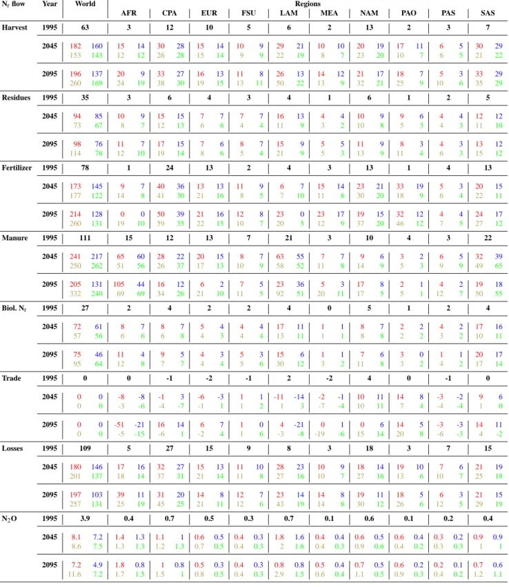
year. In the A2 scenario the loss even continues at low rates until the end of the century. The reduced inputs of soil or-ganic matter loss have to be replaced by inoror-ganic fertilizers. Our estimates of inorganic fertilizer consumption are within the range of previous estimates. Figure 3 compares our results to estimates by Daberkow et al. (2000), Davidson (2012), Erisman et al. (2008), Tilman et al. (2001), Tubiello and Fischer (2007) and Bouwman et al. (2009). The differ-ences in estimates is enormous, ranging in 2050 from 68 (Bouwman et al., 2009) to 236 Tg Nr(Tilman et al., 2001). In
150
1965 1975 1985 1995 2005 2015 2025 2035 2045 2055 2065 2075 2085 2095 0
50 100 200 250 300
Tg
N
r yr
-1
A1-MAgPIE A1-Erisman (2008)
A2-MAgPIE A2-Erisman (2008)
B1-Erisman (2008) B1-MAgPIE
B2-Erisman (2008) B2-MAgPIE
1 Davidson (2012) Inorganic fgrtilizgr
IFA (2011)
2 Daberkow et al. (2000)
3 Tilman et al. (2001)
4 Tubiello and Fischer (2007) Bouwman et al. (2009)
5 1 1
3
3
2 2 2
4
5 55 2
5 5 5 5
Fig. 3. Fertilizer consumption: historic dataset of IFADATA (2011), SRES scenario estimates by Erisman et al. (2008), Bouwman et al.
(2009), Tubiello and Fischer (2007) and our study, as well as other estimates by Davidson (2012), Daberkow et al. (2000) and Tilman et al. (2001).
rooted in a different scenario parametrisation and a different methodological approach: Our scenarios assume a strong de-mand increase also for relatively low income growth as we explained in Sect. 4.2. At the same time, low income growth goes along with slow efficiency improvements in production. The combined effects explain the strong rise of inorganic fer-tilizer consumption in the A2 scenario. At the same time, our estimates are based on a top-down approach, compared to the bottom-up approach of Bouwman et al. (2009, 2011) or Daberkow et al. (2000). Both approaches have advantages and disadvantages. Data availability for bottom-up estimates of fertilizer application is currently poor, and may be biased by crop-rotations and different manure application rates. Our top-down approach has the disadvantage that it has to rely on an exogenous path for the development of Nruptake
ef-ficiency. Also, as the closing entry of the budget, it accumu-lates the errors of other estimated Nrflows. But the top-down
approach has the advantage that it can consistently simulate substitution effects between different Nrsources or a change
in crop composition. This is of special importance if one sim-ulates large structural shifts in the agricultural system like an increasing importance of the livestock sector.
Data on historic fertilizer consumption is provided by IFA-DATA (2011) and FAOSTAT (2011). Both estimates diverge, as they use different data sources and calendar years. On a regional level, differences can be substantial. FAO’s esti-mate for fertilizer consumption in China in the year 2002 is 13 % higher than the estimate by IFA. As IFADATA (2011) provides longer continuous time series, we will refer to this dataset in the following. Fertilizer consumption between 1995 and 2009 (IFADATA, 2011) grows by +1.8 % per year. The estimates of Daberkow et al. (2000) and Bouwman et al. (2009, 2011) show lower growth rates of−0.4 % to +1.7 % over the regarded period of 20 to 50 yr. Our 50 yr average growth rate also stays with +0.9 % (B1) to +1.7 % (A2) below the observations. Yet, our short-term growth rate from 1995
to 2005 captures the observed development with a range of +1.5 % (B1) to +2.4 % (A2) between the scenarios. Due to trade our regional fertilizer projections are more uncertain than the global ones (see Sect. 4.2). Our results still meet the actual consumption trends of the last decades for most re-gions. However, fertilizer consumption in India rises slower than in the past or even stagnates, while the Pacific OECD region shows a strong increase in fertilizer consumption.
The range of our scenario outcomes is large for all Nr
flows, and continues to become larger over time. It can be observed that the assumptions on which the globalised and environmentally oriented scenarios are based lead to a sub-stantially lower turnover of the Nr cycle than the regional
fragmented and economically oriented scenarios.
4.4 The importance of the livestock sector
The agricultural Nrcycle is dominated by the livestock
sec-tor. According to our calculations, livestock feeding appro-priates 40 % (25 Tg) of Nr in global crop harvests and one
third (11 Tg) of Nr in aboveground crop residues.
Conver-sion byproducts add another 13 Tg Nrto the global feed mix.
Moreover, 70 Tg Nrmay be grazed by ruminants on pasture
land, even though this estimate is very uncertain due to poor data availability on grazed biomass and Nrcontent of grazed
pasture. The feed intake of 123 Tg results in solely 8 Tg Nrin
livestock products.
More efficient livestock feeding will not necessarily re-lieve the pressure from the Nrcycle. Although the trend
to-wards energy efficient industrial livestock feeding may re-duce the demand for feed, this also implies a shift from pas-ture grazing, crop residues and conversion byproducts to-wards feedstock crops. Pasture grazing and crop residues do not have the required nutrient-density for highly productive livestock systems (Wirsenius, 2000). According to our cal-culations, conversion byproducts today provide one fourth of the proteins fed to animals in developed regions. Latin America exports twice as much Nrin conversion byproducts
as in crops. At the same time, Europe cannot settle its con-version byproduct demand domestically. Concon-version byprod-ucts will not be sufficiently available if current industrialised feeding practices are adopted by other regions. The feedstock crops required to substitute conversion byproducts, pasture and crop residues will put additional pressure on the crop-land Nr flows. The pressure on pasture however will most
likely be only modest.
4.5 The future expansion of Nrpollution
All Nrthat is not recycled within the agricultural sector is a
potential environmental threat. Bouwman et al. (2009) esti-mate that over the next 50 yr, only 40–60 % of the lost Nrwill
be directly denitrified. The remaining Nrwill either volatilise
in the form of N2O, NOxand NHyor leach to water bodies.
With the surge of the Nr cycle, air, water and atmospheric
pollution will severely increase, which has strong negative consequences for human health, ecosystem services and the stability of ecosystems.
Along with local and regional impacts, it is still under de-bate whether a continuous accumulation of Nrcould
destabi-lize the earth system as a whole (Rockstr¨om et al., 2009a,b). While there is little evidence supporting abrupt changes on a global level, Nr pollution contributes gradually to global
phenomena such as biodiversity loss, ozone depletion and global warming. For the latter two, N2O emissions play a
crucial role. N2O, is currently the single most important
ozone depleting substance, as it catalyses the destruction of stratospheric ozone (Ravishankara et al., 2009). In addition, N2O has an extraordinarily long atmospheric lifetime and
absorbs infrared radiation in spectral windows not covered by other greenhouse gases (Vitousek et al., 1997). Fortu-nately, the greenhouse effect of N2O might be offset by NOx
and NHyemissions. By reducing the atmospheric lifetime of
CH4, scattering light and increasing biospheric carbon sinks,
these emissions have a cooling effect (Butterbach-Bahl et al., 2011).
According to our calculations, N2O emissions from
man-aged soils and manure contributed 3.9 Tg N2O-N, or
approxi-mately half of total anthropogenic N2O emissions (Vuuren et
al., 2011). However, the uncertainty involved is high. The re-sult of our Monte Carlo variation of the emission parameters suggests that the emissions may lie with a 90 % probability
in the range of 3.0 to 4.9 Tg N2O-N. This only covers parts of
the uncertainty, as the underlying activity data is also uncer-tain. Finally, actual agricultural emissions should be slightly higher than our estimate, as we do not cover all agricultural N2O emission sources of the National Greenhouse Gas
In-ventories (Eggleston et al., 2006) and as also these invento-ries have no full coverage. Crutzen et al. (2008), using a top-down approach, estimate total agricultural N2O emissions in
2000 to be in the range of 4.3 to 5.8 Tg N2O-N, which is
mod-estly higher than our estimate of 3.4 to 5.5 (90 % confidence, mean: 4.4) Tg N2O-N in the year 2000.
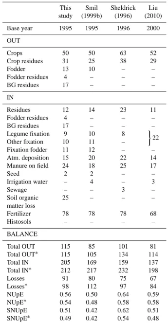
Compared to the SRES marker scenarios (Nakicenovic et al., 2000), our results suggest that emissions will increase with substantially higher growth rates in the first half of the century. Especially in the case of the A1 and B2 scenar-ios, we come to 66 % (A1) and 36 % (B2) higher cumula-tive emissions over the century. In scenario A2 our estimates are continuously approximately 20 % lower (A2), while in the B1 scenario cumulative emissions are 6 % higher (B1) but occur later in the century (Fig. 3). None of our agri-cultural N2O emission scenarios would be compatible with
the RCP2.6 scenario, which keeps the radiative forcing be-low 2.6 W
m2 in 2100 (Moss et al., 1998). To reach a
sustain-able climate target, explicit GHG mitigation efforts would therefore be required even in optimistic scenarios. If the non-agricultural N2O emissions grow in similar pace than
agri-cultural N2O emissions, the A2 scenario might even outpace
the RCP8.5 scenario.
In the beginning of the century, the uncertainty of emission parameters is much larger than the spread of scenario mean values. Only in the second half of the century, the differences of the scenarios are of similar magnitude to the emission pa-rameter uncertainty. While the scenarios are just represen-tative pathways and have no pretension to cover a specific probability space, this still indicates that a better represen-tation of the underlying biophysical processes would largely improve our emission estimates.
5 Conclusions
The current state of the global agricultural Nrcycle is highly
inefficient. Only around half of the Nr applied to cropland
soils is taken up by plants. Furthermore, only one tenth of the Nrin cropland plant biomass and grazed pasture is
actu-ally consumed by humans. During the 21st century, our sce-narios indicate a strong growth of all major flows of the Nr
cycle. In the materialistic, unequal and fragmented A2 sce-nario, inorganic fertilizer consumption more than triples due to a strong population growth and slow improvement in Nr
1960 1980 2000 2020 2040 2060 2080 2100
0 2 4 6 8 10 12 14 16
EDGAR
Tg
N
2O
-N
yr
-1
1
18
A1-MAgPIE A1B-AIM
A2-MAgPIE A2-ASF
B1-IMAGE B1-MAgPIE
B2-MESSAGE B2-MAgPIE
Crutzen et al.
Fertilized soils and
manure
Total N2O
RCP8.5 RCP2.6 Historical
1
Fig. 4. Total anthropogenic N2O emissions: historic emissions, highest and lowest RCP scenarios (Vuuren et al., 2011). N2O emissions from soils and manure: historic estimates for 1970–2008 of the EDGAR 4.2 database (EC-JRC/PBL, 2011), a top-down estimate by Crutzen et al. (2008) for the year 2000, the SRES marker scenarios (Nakicenovic et al., 2000) for 1990–2100 and our scenarios for the SRES storylines for 1995–2095. The shaded areas represent a 90 % probability range in respect to the uncertainty of emission parameters of our A2 and B1 scenarios. Our A1 and B2 scenarios have a similar relative uncertainty range.
environmentally oriented B2 scenario, food demand is lower, especially in the first half of the century. However, the live-stock sector productivity is improving only slowly and re-quires high amounts of Nrin feed. Finally, even in the
glob-alised, equitable, environmental B1 scenario, Nrin harvested
crops more than doubles and fertilizer consumption increases by 60 % and emissions by 23 % until the end of the century, with a peak in the middle of the century. In this scenario, the low meat consumption and large Nrefficiency
improve-ments both in livestock and crop production are outbalanced by population growth and the catch-up of the less developed regions with the living standard of the rich regions.
Losses to natural systems will also continuously increase. This has negative consequences on both human health and local ecosystems. Moreover, it threatens the earth system as a whole by contributing to climate change, ozone depletion and loss of biodiversity. Nrmitigation is therefore one of the
key global environmental challenges of this century. Our model of the agricultural sector as a complex interre-lated system shows that a large variety of dynamics influence Nr pollution. Each process offers a possibility of change,
such that mitigation activities can take place not only where pollution occurs physically, but on different levels of the agri-cultural system: (a) already at the household level, the con-sumer has the choice to lower his Nr footprint by
replac-ing animal with plant calories and reducreplac-ing household waste (Popp et al., 2010; Leach et al., 2012); (b) substantial wastage during storage and processing could be avoided (Gustavsson et al., 2011); (c) information and price signals on the envi-ronmental footprint are lost within trade and retailing, such that sustainable products do not necessarily have a market advantage (Schmitz et al., 2012); (d) livestock products have
potential to be produced more efficiently, both concerning the amount of Nrrequired for one ton of output and the
composi-tion of feed with different Nrfootprints; (e) higher shares of
animal manure and human sewage could be returned to farm-lands (Wolf and Snyder, 2003); (f) nutrient uptake efficiency of plants could be improved by better fertilizer selection, tim-ing and plactim-ing, as well as enhanced inoculation of legumes (Herridge et al., 2008; Roberts, 2007); (g) finally, unavoid-able losses to natural systems could be directed or retained to protect vulnerable ecosystems (Jansson et al., 1994).
Appendix A
Extended methodology
A1 Model of Agricultural Production and its Impact on the Environment (MAgPIE): general description
MAgPIE is a global land-use allocation model which is linked with a grid-based dynamic vegetation model (LPJmL) (Bondeau et al., 2007; Sitch et al., 2003; Gerten et al., 2004; Waha et al., 2012). It takes into account regional economic conditions as well as spatially explicit data on potential crop yields and land and water constraints, and derives specific land-use patterns, yields and total costs of agricultural pro-duction for each grid cell. The following will provide only a brief overview of MAgPIE, as its implementation and vali-dation is presented in detail elsewhere (Lotze-Campen et al., 2008; Popp et al., 2010, 2012; Schmitz et al., 2012).
contains 500 cluster cells, which are aggregated from 0.5 grid cells based on an hierarchical cluster algorithm (Diet-rich, 2011). Each cell has individual attributes concerning the available agricultural area and the potential yields for 18 different cropping activities derived from the LPJmL model. The geographic grid cells are grouped into ten economic world regions (Fig. 1). Each economic region has specific costs of production for the different farming activities de-rived from the GTAP model (Schmitz et al., 2010).
Food demand is inelastic and exogenous to the model, as described in further detail in the Sect. A4. Demand distin-guishes between livestock and plant demand. Each calorie demand can be satisfied by a basket of crop or livestock products with fixed shares based on the historic consump-tion patterns. There is no substituconsump-tion elasticity between the consumption of different crop products.
The demand for livestock calories requires the cultivation of feed crops. Weindl et al. (2010) uses a top-down approach to estimate feed baskets from the energy requirements of livestock, dividing the feed use from FAOSTAT (2011) be-tween the five MAgPIE livestock categories.
Two virtual trading pools are implemented in MAgPIE which allocate the demand to the different supply regions. The first pool reflects the situation of no further trade liberal-isation in the future and minimum self-sufficiency ratios de-rived from FAOSTAT (2011) are used for the allocation. Self-sufficiency ratios describe how much of the regional agri-cultural demand quantity is produced within a region. The second pool allocates the demand according to comparative advantage criteria to the supply regions. Assuming full liber-alisation, the regions with the lowest production costs per ton will be preferred. More on the methodology can be found in Schmitz et al. (2012).
The non-linear objective function of the land-use model is to minimise the global costs of production for the given amount of agricultural demand. For this purpose, the opti-mization process can choose endogenously the share of each cell to be assigned to a mix of agricultural activities, the share of arable land left out of production, the share of non-arable land converted into cropland at exogenous land conversion costs and the regional distribution of livestock production. Furthermore, it can endogenously acquire yield-increasing technological change at additional costs (Dietrich, 2011). For future projections, the model works in time steps of 10 yr in a recursive dynamic mode, whereby the technology level of crop production and the cropland area is handed over to the next time step.
The calculations in this paper are created with the model-revision 4857 of MAgPIE. While a mathematical description of the core model can be found in the Supplement, the fol-lowing Sects. A2, A3 and A4 explain the model extensions which are implemented for this study. The interface between the core model and the nutrient module consists of crop-land area (Xareat,j,v,w), crop and livestock dry-matter
produc-tion (P(xt)prodt,i,k) and its use (P(xt)dst,i,k,u). All parameters are
described in Table A2. The superscripts are no exponents, but part of the parameter name. The arguments in the sub-scripts of the parameters include most importantly time (t), regions (i), crop types (v) and livestock types (l) (Table A1).
A2 Crop residues and conversion byproducts
A2.1 Crop residues
Eggleston et al. (2006) offer one of the few consistent datasets to estimate both aboveground (AG) and below-ground (BG) residues. Also, by providing crop-growth func-tions (CGF) instead of fixed harvest indices, it can well de-scribe current international differences of harvest indices and also their development in the future. The methodology is thus well eligible for global long-term modelling. Eggleston et al. (2006) provide linear CGFs with positive intercept for cere-als, leguminous crops, potatoes and grasses. As no values are available for the oilcrops rapeseed, sunflower, and oilpalms as well as sugar crops, tropical roots, cotton and others, we use fixed harvest indices for these crops based on (Wirsenius, 2000; Lal, 2005; Feller et al., 2007). If different CGFs are available for crops within a crop group, we build a weighted average based on the production in 1995. The resulting pa-rameters rvcgf i,r
cgf s
v andr
cgf r
v are displayed in Table A3.
The AG crop residue production P(xt)prod agt,i,v is calculated as
a function of harvested production P(xt) prod
t,i,vand the physical
areaXareat,j,v,w, and BG crop production as a function of total aboveground biomass.
P(xt)prod agt,i,v := X
j∈Ii,w
Xareat,j,v,w·rvcgf i (A1)
+P(xt) prod t,i,v·r
cgf s v
P(xt)prod bgt,i,v :=(P(xt)prodt,i,v+P(xt)prod agt,i,v )·r cgf r
v (A2)
While it is assumed that all BG crop residues remain on the field, the AG residues are assigned to four different categories: feed, on-field burning, recycling and other uses. Residues fed to livestock (P(xt)ds agt,i,v,feed) are calculated based
on livestock production and livestock and regional specific residue feed basketsrt,i,l,vfb ag from Weindl et al. (2010). The de-mand rises with the increase in livestock production P(xt)prodt,i,l
and can be settled either by residues P(xt) ds ag
t,i,v,feedor by
addi-tional feedstock crops P(xt)dst,i,l,v,sag. The latter prevents that
crops are produced just for their residues.
X
v
P(xt)ds agt,i,v,feed= X
l,v
(P(xt)prodt,i,l ·rt,i,l,vfb ag (A3) −P(xt)dst,i,l,v,sag)
Residue burning (P(xt) ds ag
t,i,v,burn) is fixed to 15 % of total AG