PAIRWISE LINKAGE FOR POINT CLOUD SEGMENTATION
Xiaohu Lu, Jian Yao∗, Jinge Tu, Kai Li, Li Li, Yahui Liu
School of Remote Sensing and Information Engineering, Wuhan University, Wuhan, Hubei, P.R. China (xiaohu.lu,jian.yao,kaili,li.li,liuyahui)@whu.edu.cn
http://cvrs.whu.edu.cn/
Commission III, WG III/2
KEY WORDS: Pairwise Linkage, Clustering, Point Cloud Segmentation, Slice Merging
ABSTRACT:
In this paper, we first present a novel hierarchical clustering algorithm named Pairwise Linkage (P-Linkage), which can be used for clustering any dimensional data, and then effectively apply it on 3D unstructured point cloud segmentation. The P-Linkage clustering algorithm first calculates a feature value for each data point, for example, the density for 2D data points and the flatness for 3D point clouds. Then for each data point a pairwise linkage is created between itself and its closest neighboring point with a greater feature value than its own. The initial clusters can further be discovered by searching along the linkages in a simple way. After that, a cluster merging procedure is applied to obtain the finally refined clustering result, which can be designed for specialized applications. Based on the P-Linkage clustering, we develop an efficient segmentation algorithm for 3D unstructured point clouds, in which the flatness of the estimated surface of a 3D point is used as its feature value. For each initial cluster a slice is created, then a novel and robust slice merging method is proposed to get the final segmentation result. The proposed P-Linkage clustering and 3D point cloud segmentation algorithms require only one input parameter in advance. Experimental results on different dimensional synthetic data from 2D to 4D sufficiently demonstrate the efficiency and robustness of the proposed P-Linkage clustering algorithm and a large amount of experimental results on the Vehicle-Mounted, Aerial and Stationary Laser Scanner point clouds illustrate the robustness and efficiency of our proposed 3D point cloud segmentation algorithm.
1. INTRODUCTION
Segmentation is one of the most important pre-processing step for automatic processing of point clouds. It is a process of classi-fying and labeling data points into a number of separate groups or regions, each corresponding to the specific shape of a surface of an object. The cluster analysis which classifies elements into cat-egories according to their similarities has been applied in many kinds of fields, such as data mining, astronomy, pattern recog-nition, and can also be applied on the segmentation of 3D point clouds.
1.1 Point Cloud Segmentation
Segmentation in 3D point clouds obtained from laser scanners is not trivial, because the three dimensional point data are usually incomplete, sparsely distributed, and unorganized, also there is no prior knowledge about the statistical distribution of the points, and the densities of points vary with the point distribution. Many methods have been developed to improve the quality of segmen-tation in 3D point clouds that can be classified into three main categories: edge/border based, region growing based and hybrid.
The edge/border based methods attempt to detect discontinuities in the surfaces that form the closed boundaries, and then points are grouped within the identified boundaries and connected edges. These methods usually apply on the depth map where the edges are defined as the points where the changes of the local surface properties exceed a given threshold. The local surface properties mostly used are surface normals, gradients, principal curvatures, or higher order derivatives (Sappa and Devy, 2001, Wani and Arabnia, 2003). However, due to noise caused by laser scanner-s themscanner-selvescanner-s or scanner-spatially uneven point discanner-stributionscanner-s in 3D scanner-space,
∗Corresponding author
such methods often detect disconnected edges which makes it d-ifficult for them to identify closed segments (Castillo et al., 2013) without a filling or interpretation procedure.
The region growing based approaches deal with segmentation by detecting continuous surfaces that have homogeneity geometrical properties. In the segmentation of unstructured 3D point clouds, these methods firstly choose a seed point from which to grow a region, and then local neighbors of the seed point are combined with it if they have similarities in terms of surface point proper-ties such as orientation and curvature (Rabbani et al., 2006, Ja-gannathan and Miller, 2007). There are also algorithms which take a sub window (Xiao et al., 2013) or a line segment (Harati et al., 2007) as the growth unit. (Woo et al., 2002) proposed an octree-based 3D-grid method to handle large amount of un-structured point clouds. The smoothly connected regions are the key points of the region growing based methods. Surface normal and curvatures constraints were widely used to find the smoothly connected areas (Klasing et al., 2009, Belton and Lichti, 2006). In general, the region growing based methods are more robust to noise than the edge-based ones because of the using of glob-al information (Liu and Xiong, 2008). However, these methods are sensitive to the location of initial seed regions and inaccurate estimations of the normals and curvatures of points near region boundaries can cause inaccurate segmentation results, and also outliers can result in over- and under-segmentation.
de-pends on the success of either or both of the underlying methods.
1.2 Clustering
The cluster analysis, which aims at classifying elements into cat-egories on the basis of their similarities, has been applied in many kinds of fields, such as data mining, astronomy, and pattern recog-nition. In the last several decades, thousands of algorithms have been proposed to try to find a better solution for this problem in a simple but philosophical way. In general, these algorithms can be divided into two categories: partitioning and hierarchical methods. The partitioning clustering algorithms usually classify each data point to different clusters via a certain similarity mea-surement. The traditional algorithms K-Means (MacQueen et al., 1967) and CLARANS (Ng and Han, 1994) belong to this cate-gory. The hierarchical methods usually create a hierarchical de-composition of a dataset by iteratively splitting the dataset into smaller subsets until each subset consists of only one object, for example, the single-linkage (SLink) method and its variants (Sib-son, 1973).
1.3 Clustering in Point Cloud Segmentation
The clustering algorithms which classify elements into categories on the basis of their similarities can also be applied on the seg-mentation of 3D point clouds. The widely used K-Means algo-rithm (MacQueen et al., 1967), which can divide the data points intoK(a predefined parameter that gives the number of clusters), was applied in (Lavou´e et al., 2005) to classify the point cloud-s into 5 clucloud-stercloud-s according to their curvaturecloud-s. The cloud- shortcom-ing of the K-Means clustershortcom-ing algorithm is that it needs to know the number of clusters beforehand, which can’t be predefined in many cases. To overcome this shortcoming, the mean shift algo-rithm (Comaniciu and Meer, 2002), which is a general nonpara-metric technique to cluster scattered data, was employed on the point cloud segmentation (Yamauchi et al., 2005b, Yamauchi et al., 2005a, Zhang et al., 2008). In the works of (Yamauchi et al., 2005b, Yamauchi et al., 2005a), the mean shift algorithm was employed to integrate the mesh normals and the Gaussian curva-tures, respectively. In the work of (Liu and Xiong, 2008), the normal orientation was converted into the Gaussian Sphere, and a novel cell mean shift algorithm was proposed to identify planar, parabolic, hyperbolic or elliptic surfaces in a parameter-free way. However, most of the point cloud segmentation methods based on clustering can only discover small amount segmentations, which can be employed on some industry applications but may fail on the vehicle-mounted and aerial laser scanner point clouds which contains thousands of surfaces in large indoor/outdoor scenes.
1.4 Objectives and Motivation
In this paper, we aim to develop a simple, efficient point cloud segmentation algorithm which can be applied on a large amoun-t of unsamoun-trucamoun-tured Vehicle-Mounamoun-ted, Aerial and Samoun-taamoun-tionary Laser Scanner point clouds by employing the clustering algorithm on point cloud segmentation. To achieve this goal, we introduce two algorithms:
P-Linkage Clustering: Based on the assumption that: a data point should be in the same cluster with its closest neighbor-ing point (CNP) which is more likely to be a cluster center, we propose a novel hierarchical clustering method named Pairwise Linkage (P-Linkage) which can discover the clusters in a simple and efficient way. Firstly, a pairwise linkage procedure is applied to link each data point to its CNP on the data-point level. Then the initial clusters can be discovered by searching along the pairwise linkages starting from the points with local-maximal densities.
3 2 1 0 1 2 3
0 0.05 0.1 0.15 0.2 0.25 0.3 0.35 0.4
Gaussian Propogation
P3
P1
P6
P5
P4 P2
C
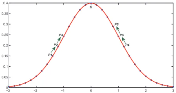
Figure 1: An illustration of the pairwise linkage on a 2D Gaus-sian curve. Derived from the non-maximum suppression, the P-Linkage compares each data point to its neighbors and forms the linkages fromp1→p2→p3...→c.
25
7 2
9 32
22 5
8
27 4
3 13
19 11 39 12
36 6 10
33
15 23
30 37 31 24 35
38 29 21 28 20
14
18 26
16
17 7
9 9
6
33 2
1
34
d
c
Figure 2: An illustration of the hierarchical clustering procedure. The data pointsp1andp34are the cluster centers, the symbol→ indicates the pairwise linkage, and the big circle in green denotes the neighborhood set of a data point with a cutoff distancedc.
The proposed clustering method is not iterative and needs only one step for general cases, and also a cluster merging method is proposed for specific cases.
Point Cloud Segmentation: Based on the proposed P-Linkage clustering, we develop a simple and efficient point cloud segmen-tation algorithm which needs only one parameter and can be ap-plied on a large amount of unstructured Vehicle-Mounted, Aerial and Stationary Laser Scanner point clouds. The P-Linkage clus-tering in point cloud segmentation takes the flatness of the esti-mated surface of a 3D point as its feature value and forms the initial clusters via point data collection along the linkages. For each initial cluster we create a slice. All the slices are merged in a simple or efficiently strategy to get the final segmentation result. The proposed point cloud segmentation algorithm needs only one parameter to balance the segmentation results of planar and surface structures.
The remainder of this paper is organized as follows. The pro-posed P-Linkage clustering algorithm is detailedly described in Section 2. The point cloud segmentation algorithm by employ-ing the P-Linkage clusteremploy-ing on 3D unstructured point clouds is introduced in Section 3. Experimental results on different kinds of synthetic and real data are presented in Section 4 followed by the conclusions drawn in Section 5.
2. PAIRWISE LINKAGE
The key conception of the P-Linkage clustering method is that: a data pointpishould be in the same cluster with its closest
neigh-borpjthat is more likely to be a cluster center, and this
relation-ship betweenpiandpjis called a pairwise linkage. This
(NMS) (Canny, 1986, Neubeck and Van Gool, 2006), in which one data point is only needed to compare with its neighbors and will be suppressed if it is not local-maximal. Figure 1 shows an illustration of the NMS, from which we can see thatp1is sup-pressed byp2 and the same suppression occurs onp2 when it is compared top3, which result in a linkp1 →p2 → p3. In this way, all the data points on the curve are finally linked to the cluster centerc,which is the local-maximal one, just via compar-ing to their neighborcompar-ing points. In fact, the P-Linkage clustercompar-ing makes up the gap between the local to the global information of the data points, which makes it more robust than the local-based clustering methods and more efficient than the global-based ones. In the following subsections, we will introduce the pairwise link-age algorithm on the clustering of 2D data points, which takes the density of a data point as its feature value to build linkages.
Cutoff Distance: The cutoff distancedc, as shown in Figure 2,
is a global parameter to demarcate the neighborhood set of a data pointpifrom other data points. In the recent work of (Rodriguez
and Laio, 2014), the value ofdcwas set as the value at the1%−
2%-th of all the distances between any two data points, denoted as the setD, which were sorted in ascent order. However it is not appropriate to set the cutoff distancedcin this way because
dc is an indicator of the distribution of the neighboring points,
and it should be derived from the local neighborhood instead of D. Thus, we propose a simple method to determine the value of dc, which is described as follows. For each data pointpi, the
distance betweenpiand its closest neighbor is recorded inDcn,
and thendcis computed as:
dc=scale×median(Dcn), (1)
wherescaleis a customized parameter which means the cutoff distancedcisscaletimes the value of the median value of the
setDcn. In this way,dcrepresents much more neighborhood
dis-tribution information than setting it1%−2%-th ofD. Only the data points whose distances topiare smaller thandcare
consid-ered as the neighborhood set ofpi, which is denoted asIi, as the
green circle shown in Figure 2.
Density: (Rodriguez and Laio, 2014) defined the density of a data pointpias the number of data points of its neighbors, which is
discrete-value and thus is not suitable for our application requir-ing continuous values for densities. In our proposed method, the densityρiof a data pointpiis calculated by applying a Gaussian
Kernel on all the data points as follows:
ρi= X
j∈[1,N],j6=iexp −(dij/dc)
2
, (2)
whereN denotes the number of all the data points anddijis the
distance between two pointspiandpj.
Pairwise Linkage: With the densities of all the data points, the pairwise linkage can be recovered in a non-iterative way, which is performed as follows. For a data pointpiwhose neighborhood
set isIi, we traverse each point inIiand find the closest data
pointpj whose density is greater than that ofpi, and then we
consider the data point pi should be in the same cluster aspj
and record the linkage between the data pointspi and pj. If
the density ofpiis local-maximal, which means that there exists
no data point inIiwhose density is greater than that ofpi, we
considerpias a cluster center. The result of the pairwise linkage
procedure is comprised of a lookup tableTrecording the linkage relationship and a setCcenterrecording all the cluster centers.
Hierarchical Clustering: The hierarchical clustering is a top-down procedure, which is similar to that of the divisive clus-tering algorithm. For each cluster centerciinCcenter, we start
searching the lookup tableTfromciin a depth-first or
breadth-first way to gather all the data points that are directly or indi-rectly connected withci, which generates a cluster whose
cen-ter isci. The whole hierarchical clustering finds the final
clus-ters C. Figure 2 shows an illustration of the hierarchical clus-tering procedure. From Figure 2, we can observe that p1 is the cluster center due to its local maximal density and there are four pairwise linkages between(p1,p13),(p13,p4),(p4,p27), and(p27,p8). Thus the hierarchical clustering is performed as p1 →p13→p4 →p27→p8. By this way, the clustering in-formation is propagated from the dense data points to the sparse ones, which is similar to the heat propagation.
Cluster Merging: When the data points are Gaussian-distributed, as shown in Figure 1, the hierarchical clustering via pairwise link-age can find the global cluster centers and recover the cluster-s quite well, but may fail in fragmented clucluster-stering recluster-sultcluster-s when there exist one or multiple local maximum(s). To deal with all the conditions of data point distribution, a customized cluster merg-ing strategy is proposed with the followmerg-ing three steps. Firstly, for each clusterCp, the average densityµpand the standard
de-viationσpof all the data points inCpare calculated. Secondly,
the adjacent clusters for each clusterCpare collected by
search-ing for the border data points between adjacent clusters. For each data pointpiinCp, its neighborhood set is denoted asIi. If a
data pointpjinIibelongs to another clusterCq, these two
clus-ters are considered to be a pair of adjacent clusclus-ters,piandpjare
recorded as the adjacent points betweenCpandCq, respectively.
Thirdly, for each adjacent cluster pairCpandCq, the average
den-sities of the adjacent points ofCpandCqare denoted asρpand
ρq, respectively. These two adjacent clusters will be merged if
the following conditions are met:
ρp> µq−σq and ρq> µp−σp. (3)
The cluster merging is conducted iteratively, which means that all the clusters that are directly or indirectly adjacent to the start cluster are merged.
Outliers: In the previous work presented by (Ester et al., 1996), the outlier points are the ones whose densities are smaller than a certain threshold. By this way, the low density data points may be classified as outliers. In the work of (Rodriguez and Laio, 2014) the outlier points are considered as those whose densities are small than the highest density in the border region of a cluster, which means that all the data points in the border region of a cluster are discarded as outliers. In our work, we consider the outliers on the cluster-level. If a data pointpiwhose density is
local-maximal but smaller than the median density, median(ρ), of all the data points, all the data points in the same cluster with piare considered as outliers.
is classified into the blue cluster, which is quite reasonable. The four data points in black,p26,p18,p17, andp16, are classified as outliers because there exist no CNP in their neighborhood, and the densities of their cluster centers are not high enough neither.
As a summary, the proposed clustering method can discover the clusters and cluster centers in only one step in general cases with-out the merging procedure. For each data pointpiwith a density
ρi, we find its closest neighboring pointCN P(pi)whose
den-sity is greater than that ofpi, and classify the point pi to the
same cluster asCN P(pi). If the densityρiof the data point
piis local-maximal and greater than the average densityρ, we
considerpias a cluster center. Algorithm 1 describes the
com-plete procedure in details of the proposed P-Linkage clustering method.
Algorithm 1Hierarchical Clustering by Pairwise Linkage Require: The density of each data point; the cutoff distancedc.
Ensure: The clustersC; their cluster centersCcenter.
1: ρi: the density of a data pointpi
2: ρ: the average density of all the data points 3: Ii: the neighborhood set of a data pointpi
4: T: the lookup table recording all the pairwise linkages 5: for eachdata pointpido
6: SetLocalMaximal←TRUE
7: Setdmin← ∞andCN P(pi)← ∅
8: for eachneighboring pointpjinIido
9: Setdij←the distance betweenpiandpj
10: ifρj> ρianddij< dminthen
11: SetLocalMaximal←FALSE
12: SetCN P(pi)←pj,dmin←dij
13: end if 14: end for
15: if NOTLocalMaximal then
16: Record the linkage betweenpiandCN P(pi)intoT
17: else ifLocalMaximalandρi>median(ρ)then
18: Insert the data pointpiintoCcenter
19: end if 20: end for
21: Collect the clustersCby searching data points in the lookup tableTfrom each data point inCcenter
3. P-LINKAGE FOR POINT CLOUD SEGMENTATION The segmentation of point clouds can also be formulated as a clustering problem because the data points on a small surface of-ten share the similar normal value. Thus we can employ the pro-posed P-Linkage clustering method on the segmentation of point clouds, which differs from that on the 2D data points in three as-pects: (1) the neighborhood is based on theKnearest neighbors (KNN) instead of the fixed distance neighbors; (2) the feature value is the flatness of the estimated surface instead of the den-sity of neighbors; (3) the distance of two data point is measured as the deviation of their normal orientations instead of their Eu-clidean distance. In the following subsections we will explain the P-Linkage based point cloud segmentation algorithm in details.
Normal Estimation: The normal for each point is estimated by fitting a plane to some neighboring points. This neighborhood can be specified in two different methods: Knearest neighbors (KNN) based and Fixed distance neighbors (FDN) based. For each data point, the KNN based methods select theK points from the point clouds having the minimum distance to it as its neighborhood, which is usually achieved by applying space par-titioning strategies like the k-d tree (Arya et al., 1998). The FDN
based methods (Toth et al., 2004) select all the points within a distance to each point, and thus the number of neighbors changes according to the density of the point clouds. Compared to KNN, the number of neighbors of FND is less in the areas of low densi-ty area, which may result in inaccurate estimation of the normals. In this paper, we employ the KNN method to find the neighbors of each data point and estimate the normal of the neighboring sur-face via the Principal Component Analysis (PCA). The procedure contains three following steps. Firstly, we build a k-d tree by ap-plying the ANN library (Mount and Arya, 2010). For each data pointpi, itsKnearest neighbors (KNN) is found and recorded as
Iiwhich is sorted in ascending order according to their distances
topi. Secondly, for each data pointpi, the covariance matrix is
formed by the firstK/2data points in its KNN setIias follows:
Σ= 1
K/2
XK/2
i=1(pi−p)(pi−p)
T,
(4)
whereΣdenotes the3×3covariance matrix andprepresents the mean vector of the firstK/2data points inIi. Then the standard
eigenvalue equation:
λV=ΣV (5)
can be solved using Singular Value Decomposition (SVD), where Vis the matrix of eigenvectors (Principal Components, PCs) and λ is the matrix of eigenvalues. The eigenvectorsv2, v1, and v0inVare defined according to the corresponding eigenvalues sorted in descending order, i.e.,λ2 > λ1 > λ0. The first two PCsv2andv1form an orthogonal basis which indicate the two dimensions of highest variability that defines the best fitted plane of the neighboring points inIi, the third PCv0 is orthogonal to the first two PCs, and approximates the normal of the fitted plane. λ0estimates how much the points deviate from the tangent plane which can evaluate the quality of a plane fitting, and the smaller the value ofλ0the better the quality of the plane fitting.
For each data point, we first find its K nearest neighbors and calculate its eigenvectors via the firstK/2neighbors via PCA, and then take the eigenvector v0 as the normal and the eigen-valueλ0 as the flatness of the estimated plane. After that, the Maximum Consistency with Minimum Distance (MCMD) algo-rithm (Nurunnabi et al., 2015) is employed to find the inliers and outliers, which is conducted as follows. First, the orthogonal dis-tances{dk
o}Kk=1for theKnearest neighbors of a data pointpi
to its estimated plane are calculated, which are collected as a set NOD={dko}Kk=1. Then, the Median Absolute Deviation (MAD) is calculated as follows:
M AD=a×mediandk o∈NOD|d
k
o−median(NOD)|, (6)
where median(NOD)is the median value ofNODanda= 1.4826
is set constant. The inliers, also known as the Consistent Set (CS), are those data points whoseRzscores:
Rz=|
dk
o−median(NOD)|
M AD (7)
are less than a constant threshold 2.5 (Nurunnabi et al., 2015). Thus for each data pointpi, we obtain its normaln(pi), flatness
λ(pi)and Consistent SetCS(pi).
Linkage Building: With the normals, flatnesses andCSs of all the data points, the pairwise linkage can be recovered in a non-iterative way, which is performed as follows. For each data point piwe search in itsCSto find out the neighbors whose flatnesses
are smaller than that ofpiand choose the one among them whose
normal has the minimum deviation to that ofpiasCN P(pi). If
there exitsCN P(pi), a pairwise linkage betweenCN P(pi)and
λ(pi)ofpiis the minimum one in its neighborhood andλ(pi)
is smaller than the following threshold:
thλ=λ+σλ, (8)
whereλis the average value of the flatnesses of all theN data
points,σλ = q
PN
i=1(λ(pi)−λ)2/N is standard deviation of all the flatnesses, thus we takepias a cluster center, and insert it
into the list of cluster centersCcenter.
Slice Creating: To create the surface slices, the clustersC are firstly formed by searching along the lookup tableTfrom each cluster center inCcenterto collect the data points that are
direct-ly or indirectdirect-ly connected with it. The clusters whose numbers of data points are smaller than 10 will be removed as outliers. Then for each clusterCpa slice is created by plane fitting via the
MCS method proposed by (Nurunnabi et al., 2015), which is an iterative procedure with the iteration number calculated as:
It= log(1−P)
log(1−(1−ǫ)h0), (9)
whereh0 is the size of the minimal subset of the data points in Cpwhich equals to 3 for plane fitting,Pis the probability of the
event that there exists at least one case in all theItiterations that
the random chosenh0minimal subset is outlier free, andǫis the outlier rate inCpwhich was set50%for general cases. Then for
each iteration in the MCS method, the following steps are per-formed: (1) First,h0 data points are chosen randomly. (2) For theh0-subset, a plane is fitted via the PCA, and the orthogonal distance for all the data points inCpare calculated and recorded
inNOD. (3) ThenNODis sorted in ascending order and the firsth
(hequals to half the size ofCp) data points are chosen to form the
h-subset. (4) Finally, the PCA is applied again on theh-subset to fit for a plane whose flatnessλ0is added into the list of previ-ous flatnesses, defined as the setS(λ0). After the iterations, the S(λ0)is sorted in ascending order, and the plane corresponding to the smallest flatness is chosen to be the best fitted plane ofCp.
Then the MCMD outlier removal method is applied to find out the inliers, also known as the Consistent Set (CS), to the best fitted plane inCp. Thus for each sliceSp, we obtain its normal
n(Sp), flatnessλ(Sp) and Consistent SetCS(Sp)in the same
way as each data point.
Slice Merging: To obtain complete planar and curved surfaces which are quite common in the indoor and industry applications, a normal and efficient slice merging method is proposed, which is similar to the Cluster Merging procedure introduced in the P-Linkage clustering and contains the following steps. First, we search for the adjacent slices for each one, two slicesSpandSq
are considered adjacently if the following condition is satisfied:
∃ pi∈CS(Sp) and pj∈CS(Sq),
where pi∈CS(pj) and pj∈CS(pi).
(10)
Then, for a sliceSpand one of its adjacent sliceSq, they will be
merged if the following condition is satisfied:
arccos n(Sp)
⊤ ·n(Sq)
< θ, (11)
wheren(Sp)andn(Sq)are the normals ofSpandSq,
respec-tively, andθis the threshold of the angle deviation. The greaterθ is, the more curving the surface can be. The slice merging is con-ducted iteratively, which means that all the slices that are directly or indirectly adjacent to the start slice will be processed.
(a)scale= 5 (b)scale= 5
Figure 3: Clustering results of the proposed method on the Gaus-sian distributed test data.
4. EXPERIMENTAL RESULTS 4.1 Evaluation on Clustering
The only customized parameter the P-Linkage requires is thescale used to determine the value ofdc. We setscale= 5for
gener-al cases, which will be proved in the following experiments to be a good choice. The merging procedure, which is specifically designed for the uniform distribution data, is not in use in gener-al case but can be customized to get a better result if the initigener-al clustering result contains too much fragments.
To evaluate the proposed method on the Gaussian distribution da-ta, we chose two test data in the “Shape sets”1, which contain 15 and 31 clusters, respectively. Figure 3 shows the clustering re-sults on them, where the black points stand for the outliers, and the points in other different colors belong to different clusters. We can see that, in both data sets, all the clusters were correct-ly discovered, and the outliers extracted by the proposed method were all reasonable to be picked out. In both cases, the value of scalewas set as 5.
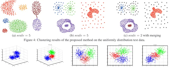
To further evaluate the proposed method on the uniformly distri-bution data, the two other test data in the “Shape sets” were test-ed. Figure 4 shows the clustering results of our method. In Fig-ure 4(a) all the 7 clusters were discovered and distinguished well. While in Figure 4(b), the left-down data points in purple were all classified into a single cluster, the reason is that thescale= 5is too large for this case. By reducingscale= 2and applying the merging procedure, a better clustering result can be achieved in Figure 4(c), however in this condition more data points were dis-carded as outliers (points in black) because there are not enough data points in its neighborhood thus the densities are smaller than the density threshold to be a new cluster.
We also tested the P-Linkage method on multi-dimensional data sets to see its robustness. Figure 5 shows the clustering result on a simulated 3D data which is composed of three subsets in Gaussian distribution. Each subset contains 200 data points. The number of correct classified data points for each subset is 175 (87.5%), 195 (97.5%) and 191 (95.5%), respectively. In all the three 2D views in Figure 5, we can see that all the three subsets were divided well.
4.2 Evaluation on Point Cloud Segmentation
Unlike the traditional K-Means algorithm and the approach pro-posed by (Rodriguez and Laio, 2014), the propro-posed P-Linkage clustering can be employed directly on the applications like point cloud segmentation where there exist a huge amount of clusters of data points in complex scenes. To test the robustness of the pro-posed point cloud segmentation method, we applied it on Vehicle-mounted, Aerial and Stationary Laser Scanner point clouds. In all
(a)scale= 5 (b)scale= 5 (c)scale= 2with merging Figure 4: Clustering results of the proposed method on the uniformly distribution test data.
−4 −2
0 2
4
−2 0 2 4 −4 −2 0 2 4
−4 −2
0 2
4
−2 0 2 4 −3 −2 −1 0 1 2 3
XYZ−view
−3 −2 −1 0 1 2 3 −1.5
−1 −0.5 0 0.5 1 1.5 2 2.5 3
XY−view
−1.5 −1 −0.5 0 0.5 1 1.5 2 2.5 3 −3
−2 −1 0 1 2 3
YZ−view
−3 −2 −1 0 1 2 3 −3
−2 −1 0 1 2 3
XZ−view
Figure 5: Clustering results of the proposed method on the 3D (XY Z) simulated test data: the original data points and the clustering result projected onto theXY plane, theY Zplane, and theXZplane from left to right.
these tests, only the parameterθwas adjusted to get the best seg-mentation results without any filtering or diluting.
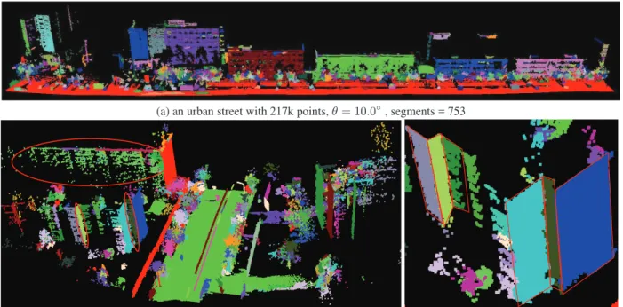
Vehicle-mounted: The segmentation of dense vehicle-mounted laser scanner points is a challenging task due to the existence of varied kinds of road furnitures which contain signs and light poles, road barricades, billboards, the ground and vehicles. In this work, two vehicle-mounted datasets were tested as shown in Figure 6(a) captured from an urban street of 355 meters long with 217k points and in Figure 6(b) captured from a small partial of a city in details containing 120k points. From Figure 6(a) contain-ing road, buildcontain-ings, street lamps, vehicles and trees, we observe that the road surface was clustered into a complete one and sepa-rated entirely from other objects. Also, the building facades were discovered quite well. From Figure 6(b), we observe that most of the building facades were segmented well despite that their densities vary in a wide range. Those facades perpendicular to the road (the green slice within the big red ellipse frame) and the small slices connected with other big ones (the two slices with-in the small red ellipse frames) were recovered quite well. Fig-ure 6(c) shows a detailed look of the segmentation result with the red quadrangles representing different slices, which means that the segmentation result of the proposed method can be applied on the extraction of street patches with more specific operations.
Aerial: The first aerial data set tested is composed of 3433k points, which covers an urban area of 5km×5km. There are buildings, ground, road and vegetations in this data set. Fig-ure 7(a) shows a partial result of the whole data set, from which we can see that the ground was separated by the road (left bottom, in orange) into two parts, in purple and lemon yellow, respective-ly, and the ground in purple was segmented into a whole surface despite of the various objects on the ground. The roofs of build-ings were segmented into a whole part in general, while some small structures can also be kept. Figure 7 (b) shows a detailed view of the segmentation result of the area in red frame in Fig-ure 7(a), from which we can see that the proposed method can preserve the details well. The second tested aerial data set is the ISPRS commission III/4 benchmark on Urban Classification and 3D Building Reconstruction and Semantic Labeling2, the result-s of which are result-shown in Figure 7(c) and (d). We can result-see that the objects including the trees and building are generally sepa-rated from the ground which is segmented into a single part, and the details of the roofs are preserved well as Figure 7(d) shows.
2http://www2.isprs.org/commissions/comm3/wg4/tests.
html
More experiments to evaluate the accuracy and correctness of the segmentation method will be presented in the futrure work. What is noteworthy is that to achieve the segmentation results on both data sets, only the nearest neighbors size K in k-d tree building and theθin slices merging is adjusted.
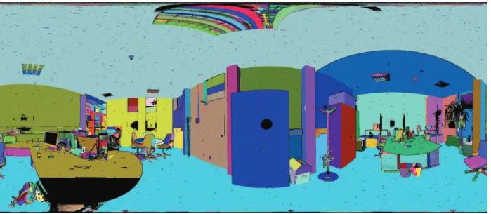
Stationary: The tested stationary laser scanner data set consists of 2500×1076 data points, which means it can be unfolded into a 2D image whose column equals 2500 and row equals 1076. Figure 8 shows the segmentation result on a 2D image, from which we can see that all the main surfaces were segmented well. Specifically, we notice that the details of the modulator tubes on the ceiling were preserved quite well. In this case we set θ= 20.0◦due to that there exist many streamlined objects in this indoor scene, which will result in more surfaces and less planes.
5. CONCLUSION
In this paper we propose a novel hierarchical clustering method named P-Linkage to discover the clusters in a simple and effi-cient way by recovering the pairwise linkages on the data point level. The proposed P-Linkage clustering can be employed di-rectly on the applications which have huge amount of clusters and complex scene. Applying the P-Linkage clustering on point cloud segmentation, we develop an efficient point cloud segmen-tation algorithm which can handle a huge amount of data points captured from different scenes. Experimental results on different dimensional synthetic data from 2D to 4D sufficiently demon-strate the efficiency and robustness of the proposed P-Linkage clustering algorithm and a large amount of experimental result-s on the Vehicle-Mounted, Aerial and Stationary Laresult-ser Scanner point clouds sufficiently illustrate the robustness and efficiency of our proposed 3D point cloud segmentation algorithm.
ACKNOWLEDGMENT
This work was supported by the National Natural Science Foun-dation of China (Project No. 41571436), the National Basic Re-search Program of China (Project No. 2012CB719904), the Jiang-su Province Science and Technology Support Program, China (Project No. BE2014866), the Hubei Province Science and Tech-nology Support Program, China (Project No. 2015BAA027), and the South Wisdom Valley Innovative Research Team Program.
REFERENCES
near-(a) an urban street with 217k points,θ= 10.0◦, segments = 753
(b) an urban region with 120k points,θ= 10.0◦, segments = 468 (c) local details of partial regions in (b) Figure 6: Segmentation results of the proposed method on the vehicle-mounted test data.
(a) urban set 1,θ= 10.0◦ (b) in details
(c) urban set 2,θ= 10.0◦ (d) in details
Figure 7: Segmentation results of the proposed method on two aerial data sets.
est neighbor searching fixed dimensions. Journal of the ACM (JACM)45(6), pp. 891–923.
Belton, D. and Lichti, D. D., 2006. Classification and segmenta-tion of terrestrial laser scanner point clouds using local variance information. International Archives of Photogrammetry, Remote Sensing and Spatial Information Sciences36(5), pp. 44–49.
Benk˝o, P. and V´arady, T., 2004. Segmentation methods for smooth point regions of conventional engineering objects.
Computer-Aided Design36(6), pp. 511–523.
Canny, J., 1986. A computational approach to edge detection.
IEEE Transactions on Pattern Analysis and Machine Intelligence
Figure 8: Segmentation results of the proposed method on the stationary indoor test data withθ= 20.0◦.
Castillo, E., Liang, J. and Zhao, H., 2013. Point cloud segmenta-tion and denoising via constrained nonlinear least squares normal estimates. In:Innovations for Shape Analysis, Springer, pp. 283– 299.
Comaniciu, D. and Meer, P., 2002. Mean shift: A robust ap-proach toward feature space analysis.IEEE Transactions on Pat-tern Analysis and Machine Intelligence24(5), pp. 603–619.
Ester, M., Kriegel, H.-P., Sander, J. and Xu, X., 1996. A density-based algorithm for discovering clusters in large spatial databases with noise. In:Proceedings of the 2nd International Conference on Knowledge Discovery and Data Mining.
Harati, A., G¨achter, S. and Siegwart, R., 2007. Fast range image segmentation for indoor 3D-SLAM. In: Intelligent Autonomous Vehicles, Vol. 6number 1, pp. 475–480.
Jagannathan, A. and Miller, E. L., 2007. Three-dimensional sur-face mesh segmentation using curvedness-based region growing approach. IEEE Transactions on Pattern Analysis and Machine Intelligence29(12), pp. 2195–2204.
Klasing, K., Althoff, D., Wollherr, D. and Buss, M., 2009. Com-parison of surface normal estimation methods for range sensing applications. In:IEEE International Conference on Robotics and Automation, IEEE, pp. 3206–3211.
Lavou´e, G., Dupont, F. and Baskurt, A., 2005. A new CAD mesh segmentation method, based on curvature tensor analysis.
Computer-Aided Design37(10), pp. 975–987.
Liu, Y. and Xiong, Y., 2008. Automatic segmentation of unorga-nized noisy point clouds based on the gaussian map. Computer-Aided Design40(5), pp. 576–594.
MacQueen, J. et al., 1967. Some methods for classification and analysis of multivariate observations. In:Proceedings of the fifth Berkeley symposium on mathematical statistics and probability.
Mount, D. M. and Arya, S., 2010. Ann: A library for approxi-mate nearest neighbor searching. https://www.cs.umd.edu/ ~mount/ANN/.
Neubeck, A. and Van Gool, L., 2006. Efficient non-maximum suppression. In: International Conference on Pattern Recogni-tion (ICPR), Vol. 3, IEEE, pp. 850–855.
Ng, R. T. and Han, J., 1994. Efficient and effective clustering methods for spatial data mining. In: Proceedings of the 20th International Conference on Very Large Data Bases.
Nurunnabi, A., West, G. and Belton, D., 2015. Outlier detection and robust normal-curvature estimation in mobile laser scanning 3D point cloud data.Pattern Recognition48, pp. 1404–1419.
Rabbani, T., van den Heuvel, F. and Vosselmann, G., 2006. Seg-mentation of point clouds using smoothness constraint. Interna-tional Archives of Photogrammetry, Remote Sensing and Spatial Information Sciences36(5), pp. 248–253.
Rodriguez, A. and Laio, A., 2014. Clustering by fast search and find of density peaks.Science344(6191), pp. 1492–1496.
Sappa, A. D. and Devy, M., 2001. Fast range image segmentation by an edge detection strategy. In:Third International Conference on 3-D Digital Imaging and Modeling, IEEE, pp. 292–299.
Sibson, R., 1973. SLINK: an optimally efficient algorithm for the single-link cluster method.The Computer Journal16(1), pp. 30– 34.
Toth, C. D., O’Rourke, J. and Goodman, J. E., 2004. Handbook of discrete and computational geometry. CRC press.
Vieira, M. and Shimada, K., 2005. Surface mesh segmentation and smooth surface extraction through region growing.Computer Aided Geometric Design22(8), pp. 771–792.
Wani, M. A. and Arabnia, H. R., 2003. Parallel edge-region-based segmentation algorithm targeted at reconfigurable multir-ing network.The Journal of Supercomputing25, pp. 43–62.
Woo, H., Kang, E., Wang, S. and Lee, K. H., 2002. A new seg-mentation method for point cloud data. International Journal of Machine Tools and Manufacture42(12), pp. 167–178.
Xiao, J., Zhang, J., Adler, B., Zhang, H. and Zhang, J., 2013. Three-dimensional point cloud plane segmentation in both struc-tured and unstrucstruc-tured environments. Robotics and Autonomous Systems61, pp. 1641–1652.
Yamauchi, H., Gumhold, S., Zayer, R. and Seidel, H.-P., 2005a. Mesh segmentation driven by Gaussian curvature. The Visual Computer21(8-10), pp. 659–668.
Yamauchi, H., Lee, S., Lee, Y., Ohtake, Y., Belyaev, A. and Sei-del, H.-P., 2005b. Feature sensitive mesh segmentation with mean shift. In: International Conference on Shape Modeling and Ap-plications, pp. 236–243.