The Hysteresis and Shear Velocity in Unsteady Flows

Journal of Applied Fluid Mechanics, Vol. 9, No. 2, pp. 839-853, 2016. Available online at www.jafmonline.net, ISSN 1735-3572, EISSN 1735-3645.

Hysteresis and Shear Velocity in Unsteady Flows

G. Bombar

Ege University, Dept. of Civil Eng., İzmir, 35100, Turkey

Corresponding Author Email: gokcen.bombar@ege.edu.tr (Received January 5, 2015; accepted March 28, 2015)

A

The shear velocity is an important parameter in characterizing the shear at the boundary in open channels and there exist methods to estimate the shear velocity in steady flows, but the application and comparison of these methods to non-uniform unsteady flows is limited. In this study, three artificial triangular-shaped hydrographs were generated where the base flow is non-uniform with fine sand bed and the shear velocity was obtained by the methods, u*SV by using the Saint-Venant equations, u*L by using the procedure given by Clauser Method,

u*P by using the parabolic law, u*UN by using the momentum equation assuming the slope of energy grade line

is equal to bed slope and u*avg by using the average velocity equation are used in this study. The stream-wise

components of velocity time series and the velocity profiles were obtained by means of an acoustic Doppler velocity meter. The variation of the shear velocity and the constant for the parabolic law with time is discussed. It is concluded that the shear velocities found by the parabolic law and the average velocity equation can be used interchangeably. Furthermore a hysteresis intensity parameter is proposed in order to examine the depth variation of hysteretic behavior of depth variation both with point velocity and average velocity. It is revealed that the more the unsteady the hydrograph the more the hysteresis both in terms of point velocity and cross-sectional mean velocity.

Keywords: Unsteady flow; Shear velocity; Hysteresis; Velocity time series; Parabolic law; Clauser method; Saint-Venant Equations.

N

A cross sectional area B channel width

Br integral constant for rough boundaries

Bs integral constant for smooth boundaries

Cu uniformity coefficient

d10 particle size at which 10% is finer

d50 median diameter of the sediment

d65 particle size at which 65% is finer

d84 particle size at which 84% is finer

dg geometric mean diameter was

F_{base Froude number at base flow conditions} F_{peak Froude number at peak flow conditions} g gravitational acceleration

h flow depth hbase base flow depth

hpeak, peak flow depth

HPSCU speed of pump in % of 1450 rpm

ks equivalent sand roughness

qbase unit discharge at base flow conditions

qpeak unit discharge at peak flow conditions

Q flow rate

Qbase discharge at base flow conditions

QFMpeak peak discharge from flow meter

QFM discharge from flow meter

Qpeak, discharge at peak flow conditions

QVM discharge from velocity measurements

QVMpeak peak discharge from velocity

uavg smt smoothed average

uavg. velocity by averaging the repetitions

um maximum velocity,

u* shear (friction) velocity

u*avg u* obtained by Eq. (14)

u*L u* estimated by Clauser Method

u*P u* estimated by the Parabolic Law

u*SV u* estimated by Saint-Venant equation

u*UN u* obtained by Eq. (3)

uz mean point velocity at z um maximum velocity

V average flow velocity Vbase base flow velocity

Vc (Vbase+Vpeak)/2

Vpeak, peak flow velocity

w instantaneous point velocity in z dir. w’ fluctuating components in z dir.

w time varying mean point velocity in z dir. x axis for stream-wise direction

z axis for vertical direction z0 reference level

 dimensionless unsteadiness parameter

 limit between inner and outer layers

R2 _{correlation coefficients.} Rh hydraulic radius

S0 channel slope

Se slope of the energy grade line

Tf falling duration based on the flow depth

TfQ falling duration based on the flow rate

Tr rising duration based on the flow depth

TrQ rising duration based on the flow rate

TrQFM rising duration based on QFM

TrQVM rising duration based on QVM

TrV rising duration based on the velocity

u instantaneous point velocity in x dir. u’ fluctuating components in x dir.

u time varying mean point velocity in x dir

 von Karman constant

 constant in parabolic law

 hysteresis intensity parameter

 shear stress

0 boundary shear stress ρ density of the water

 wake strength parameter

h hpeak - hbase QFM QFM peak - QFM base, QVM QVM peak - QVM base, T Tr + Tf V Vpeak - Vbase

FM

 total volume of water considering QFM

VM

 total volume of water considering QVM

 

 wake function

1.

I

Velocity distribution and flow parameters such as turbulence and boundary shear stress in steady flow conditions were studied widely both experimentally in laboratory and in the field (Nezu and Rodi 1986, Cardoso et al. 1989, Kırkgöz 1989, Kırkgöz and Ardıçlıoğlu 1997, Kabiri-Samani et al. 2013, Genç et al. (2015)) and numerically (Song et al. 2012, Debnath et al. 2015, Shah et al. 2015). However, in nature, unsteady flows are the most common type of open channel flows and attracted a great amount of interest for research in the field of hydraulics (Bose and Dey 2012) particularly in the furrow irrigation and in irrigation management systems (Walker and Humpherys 1983, Meselhe and Holly 1993, Kumar et al. 2002, Zhang et al. 2012).

The experiments in open channels were conducted on hydraulically rough surfaces by Tu (1991), Song and Graf (1996), Qu (2002) and Bares et al. (2008) and on smooth surfaces by Nezu et al. (1997). Tu (1991) and Qu (2002) used micro-mouline; Nezu et al. (1997) used Laser Doppler Anemometer (LDA) for point velocity measurement at various elevations on the flow depth by repeating the experiment at various times to obtain the velocity profile. Song and Graf (1996) and later Bagherimiyab (2012) used Acoustic Doppler Velocity Profiler (ADVP) (Lhermitte and Lemmin 1994) which uses ultrasonic method to obtain the velocity profile once in each sampling time. Qu (2002) worked on both fixed and mobile beds. During the rising and falling limbs of the hydrograph, the validity of logarithmic law distribution has been investigated (Nezu and Sanjou 2006). The flow features like average velocity, turbulence intensity, Reynolds stress and shear velocity (Nezu et al. 1997, Song 1994, Tu 1991, Bares et al. 2008) are the issues investigated in unsteady flow conditions which were carried out in the laboratory studies.

In order to represent the intensity of the hydrograph which can be defined as the change of flow depth or flow rate within a specified time interval, the unsteadiness parameter is used (Nezu et al. 1997).

There exist many parameters defining unsteadiness proposed by many researchers (Nezu et al. 1997; Rowinski et al. 2000, Bombar et al. 2011, Bombar 2014) such as  ;

) / /( ) / 1

( Vc h TrQ





where h=hpeak-hbase, hbase and hpeak, are the base

flow depth and peak flow depths, Vc=(Vbase+Vpeak)/2, Vbase and Vpeak, are the base flow

and peak flow average velocities, TrQ is the rising

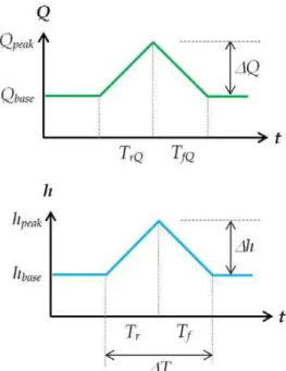
duration of the hydrograph based on the flow rate as depicted in Fig. 1. Here t is time, Q is the flow rate, Qbase and Qpeak, are the base discharge and peak

discharge, TfQ is the falling duration of the

hydrograph based on the flow rate, Q=Qpeak-Qbase,

h is the flow depth Tr and Tf are the rising and

falling durations of the hydrograph based on the flow depth and , T= Tr + Tf .

Fig. 1. Representation of the terms of a hydrograph in terms of time variation of flow

In unsteady flows it is a well-known fact that there exists a hysteresis between flow depth and mean cross sectional velocity where the velocity reaches its maximum value before the flow depth (Graf and Altınakar 1998, Nezu and Sanjou 2006). The mean velocity attains its maximum value before flow depth does (Nezu and Nakagawa 1991, Qu 2002). Song and Graf (1996), Bares et al. (2008), find out that the shear velocity attains its maximum value first and then in the order of V, Q and finally h. Qu (2002) observed that the limbs of the curve becomes farther as the unsteadiness increases. Jensen et al. (1989) investigated this time lag too (Nezu and Sanjou 2006).

According to Nezu (2005) and Nezu and Nakagawa (1993), in steady flows the shear velocity can be calculated in many ways (Lopez and Garcia 1999, Muste and Patel 1997), such as, the use of Reynolds stress graph, velocity data at the viscous sub-layer, Clauser method, parabolic law, the slope method where Saint-Venant equations are used and average velocity equation. Under unsteady flow conditions, some researchers prefer to estimate the shear stress using the depth-slope product rule corresponding to normal (steady, uniform) flow especially when the purpose of their study is to focus on overall parameters rather than local parameters (Hassan et al. 2006, Güney et al. 2013) or prefer to neglect the contribution of velocity gradient to energy slope (Powell et al. 2001). Qu (2002), Song and Graf (1996) and Afzalimehr et al. (2007) used some of these methods in unsteady flows, but the comparison of these methods is limited.

This study was carried out in the laboratory with artificial triangular-shaped hydrographs with high unsteadiness at which the base flow is non-uniform. Among the methods that have been developed to estimate the shear velocity (u*), u*SV the

Saint-Venant equations, u*L the procedure given by

Clauser Method, u*P the parabolic law and u*UN the

momentum equation assuming the slope of energy grade line is equal to bed slope and the equation for average velocity u*avg are used which are explained

below. Furthermore the hysteresis was investigated and a hysteresis intensity parameter is proposed in order to find out the depth variation of hysteretic behavior at point velocity and average velocity.

2.

T

R

The related methods are explained as follows.

1. Reynolds Stress Graph:

In uniform flows the total shear stress  varies linearly with depth as given in Eq. (2) having the value of 0 at the boundary and zero at the free surface. By linear extrapolation of the Reynolds stress profile, the shear velocity can be calculated knowing thatu* = (0/)0.5.





z u w

u' '  /  *21 /



   



where  is density, u’ and w’ fluctuating components in stream-wise direction x and vertical direction z,  is the kinematic viscosity, u is the

stream-wise component of velocity.

This method requires a high sampling frequency. In accelerating non-uniform flows the type of the graph is convex and decelerating flows it has a concave type. Muste and Patel (1997) used this method in calculating the shear velocity (or friction velocity) for flows with suspended sediment. In unsteady flow conditions, this method was used by Song and Graf (1996).

2. The slope method, Saint-Venant Equations (u*UN

& u*SV):

In steady uniform flows, from momentum balance u* is related to gravitational acceleration g, channel

slope S0 and Rh as

0

* gRS

u  _h

As the shear velocity varies around the wetted perimeter, this gives an average value of u*. For a

two-dimensional fully developed flow, or flow in a wide channel (the aspect ratio, B/h>6 where B is the channel width) h is used in place of the Rh (Muste

and Patel 1997, Graf and Altınakar 1998). Yang (2010) investigated the influence of flow geometry on the depth-average shear stress and velocity. Muste and Patel (1997) claimed that this method were of less accuracy because they incorporate errors due to piezometers and flow depth readings. The shear velocity estimated by Eq. (3) is abbreviated as u*UN:

In unsteady flows the u* becomes u* = (ghSe)1/2

where Se is the slope of energy grade line.

Saint-Venant equations consist of continuity as given in Eq. (4) and momentum equations. One can derive the latter by equating the momentum on a control volume in conservative form or in non-conservative form as given in Eq. (5a) and Eq. (5b), respectively.

0       t A x Q





1 1 0 2                    e S S g x h g A Q x A t Q A





         e S S g x h g x V V t V

where A is the cross sectional area, V is velocity and S0=-z/x. After mathematical manipulations, one

can get;                    t V g x V g V x h x z gR u h 1

*

The shear velocity estimated by Eq. (6) is abbreviated as u*SV:

3. Velocity Data at the Viscous Sub Layer:

equation given below (Lopez and Garcia 1999).



/ /u_* zu_*

u 

In unsteady flows, the velocity profile at each time instant is examined independently and the u* is

calculated for each profile, so that a time variation of u* is obtained. Onitsuka and Nezu (1999)

revealed that the linear distribution is valid both in rising and falling limbs. The drawback of the method is the limited number of data within this thin layer (Nezu and Nakagawa 1993).

4. Clauser Method (u*L):

Nikuradse (1933) has proposed a logarithmic law to describe the vertical distribution of u. The shear velocity may be obtained from the slope of the best fit line in the inner region where =z/h<0.2 (Graf and Altınakar, 1998). When u*ks/ < 5 the flow is

assumed to be smooth and the Eq. (8) is valid.

s B u z u

u _{ }



 *

* ln

1

(8)

where ks is the Nikuradse’s equivalent sand

roughness,  is the von Karman constant and equal to 0.40, Bs is the integral constant for smooth

boundaries. The rough regime occurs when u*ks/

>70 and the Eq. (9) is valid as,

r s

B k

z z u

u _  0_

* ln 1



where z0 is the reference level, Br is the integral

constant for rough boundaries. In steady flows, the ks is taken as 3.5d84 by (Leopold et al. 1964), 5d50

by (Griffiths 1981), d65 by (Wiberg and Smith 1987

and Patel and Ranga Raju 1999), 1 10d50 by Liu

(2001) for flat sand bed, 2d50 by Alabi (2006),

2.5d50 by Beheshti and Ataie-Ashtiani (2010) where

d65 and d84 are particle size at which 65% and 84%

by weight of the sample is finer, respectively, d50 is

the median diameter of the sediment. In unsteady flow experiments Song and Graf (1996) took the roughness height as d50. The reference level for a

completely rough bed was taken as 0.033ks by Jan

et al. (2006) and -0.25ks by Song and Graf (1996).

Muste and Patel (1997) claimed that this method requires 10-12 mean velocity measurements in the near-bed region for a reliable curve fit.

In the outer region, =z/h>0.2, the velocity profile deviates from the log law and could be explained by velocity defect law. As given in Eq. (10), Coles (1956) has improved the log law by introducing a wake function 

 





 

   

 

 



 s r

s

B B k

z u z u

u

, ,

ln

1 *

*

 

       

h z 2 sin

2 2 





here,  is the wake strength parameter.

Brereton et al. (1990), Tu and Graf (1992), Tardu et

al. (1994) and Song and Graf (1996) investigated the velocity profile for unsteady flows and concluded that the logarithmic law is valid in the inner region of open channel flow.

In natural channels the flow is three dimensional due to the presence of secondary currents and the measured maximum velocity occurs below the surface and this is called the velocity dip phenomenon (Guo and Julien 2008 and Guo 2014). A Modified Log-Wake Law (MLWL) is proposed by Guo and Julien (2003) and Guo et al. (2005) which is applicable to velocity data measured in both pipe and open channel flow in laboratory and field. Based on the analysis of the Reynolds-averaged Navier–Stokes (RANS) equations and a log-wake modified eddy viscosity distribution, Absi (2011) proposed an ordinary differential equation for velocity distribution to predict the velocity-dip-phenomenon. Bonakdari et al. (2008) analyzed Navier–Stokes equations and suggested a new formulation of the vertical velocity profile in the center region of steady fully developed turbulent open-channel flows. Lassabatere et al. (2013) integrated the RANS equation by assuming the variations in the transverse direction at the center of the channel could be neglected.

For unsteady flows, Nezu et al. (1997) determined that the von Karman constant is not considerably affected from the unsteadiness. The deviation of  from the value 0.41 depends on the unsteadiness parameter  and concluded that the von Karman constant was not affected from the unsteadiness and can be taken as equal to 0.41 (Onitsuka and Nezu 1999). It is proposed as 0.40 by Song and Graf (1996) and 0.41 by Brereton et al. (1990) Tardu et al. (1994), Brereton and Mankbadi (1995) and Bares et al. (2008).

The integration constant for smooth boundaries Bs

has an average value of 5 (±25%). In unsteady flows, Nezu et al. (1997) calculated the Bs as 5.3 in

the initial steady part. They find out that the value of Bs decreases in the rising limb of the hydrograph

and gets its minimum value just before the peak is reached. The Bs value increases in the falling limb

and gets it maximum value in the middle of the falling limb and then again decreases to its original steady value. Akhavan et al. (1991) and Nezu et al. (1997) obtained similar results. Onitsuka and Nezu (1999) and Nezu and Sanjou (2006) claimed that for hydrographs with small unsteadiness values (≈

0.001), the Bs remains nearly constant throughout

the hydrograph, but for the ones with higher unsteadiness, (≈ 0.0063) Bs increases in the

rising period and decreases in the falling period.

The integration constant for rough boundaries Br

has an average value of 8.5 (±15%). Song and Graf (1996) revealed that the Br parameter is equal to 8.5

as an average value. Tu and Graf (1992) calculated Br in the range of 3.8 - 14.5. Similarly Song (1994)

used the velocity data in the inner region to calculate the Br and concluded that in rising limb Br

has smaller values than the one in the falling limb.

(a)

Fig. 2. (a) Scheme of the experimental setup, (b) PSCU, (c) software of PSCU, (d) flowmeter, (e) flume computer and data logger, (f) Flow Tracker with side-looking sensors (Flow Tracker Users Manuel).

(b) (c)

(d)

(e) (f)

flow direction

measurement volume 9 mm

acoustic receiver

acoustic transmitter

the shear velocity in investigating the effect of suspended sediment flux on the velocity profile in steady flows. The slope of the linear trend line found by least square regression for u versus ln(z) is used to calculate the u*. The shear velocity

estimated by Clauser method is abbreviated as u*L:

For unsteady flows, Song and Graf (1996) find that the log law is valid in the inner region and Coles wake law is valid in the outer region the Nezu and Nakagawa (1991) mentioned that for high Reynolds numbers this deviation from log law is more prominent.

5. Parabolic Law (u*P):

The parabolic law is given by Eq. (12) and applicable for the velocity data in the outer region (Graf and Altınakar 1998).

2

*

1 

       

h z u

u u_m



where um is the maximum velocity,  is given by

the equation below (Afzalimehr et al. 2007)





 

 

1 2

5 . 2

Taking =0.2 will make the =7.8. Graf and Altınakar (1998) proposed to take  as 9.6. Kundu and Gholhal (2012) proposed to take  as 6.3 proposed by Bazin. The slope of the linear trend line between u and (1-z/h)2 _{can be used to calculate} the u*. Afzalimehr et al (2007) used this method

successfully for decelerating steady flows. The shear velocity estimated by Eq. (12) is abbreviated as u*P.

6. Average Velocity (u*avg):

The equation given below is used to calculate the shear velocity as u*avg.

25 . 6 ln

1

*

       

s h k R u

V



Recently, one and two dimensional velocity distribution in open channels is derived by maximizing the Tsallis entropy showing an advantage in capturing low velocities near the channel bed for heavy sediment flows with high entropy value (Cui and Singh 2013, Cui and Singh 2014b). Later Singh et al. (2014) derived a function for modelling the flow duration curve. Cui and Singh (2014a,c) computed the sediment discharge and sediment concentration distribution by the same method and revealed that this method has an advantage over other methods for the upper 80% depths.

3.

E

S

-

The experiments were conducted in a rectangular flume of 70 cm width, 18 m length with a bed slope of 0.004 in the Hydraulics Laboratory of Ege University, Department of Civil Engineering. The transparent sides of the flume made from plexiglass

were 50 cm high. A tail gate of 25 cm high was located at the end section. The sketch of the experimental setup is given in Fig. 2.a. The bed material used in the flume was composed of a non-uniform sediment mixture with d50 = 0.43 mm. Its

thickness was 20 cm. The geometric mean diameter was dg = 0.44 mm and geometric standard deviation

was σg = 2.27. The uniformity coefficient (Cu =

d60/d10) was 3.72. At the first 1.7 m of the flume

coarse grains were placed in order to prevent the local scour at the entrance.

The water was circulated continuously. The volume of the water supply reservoir was approximately 47 m3. The pump used in this study was capable of producing a flow rate up to 100 l/s, and it was connected to a speed-control unit (PSCU) given in Fig. 2.b that can control the flow rate by a program by increasing and/or decreasing the pump speed HPSCU (in percentage of 1450 rpm) at desired time

increments. The software window is given in Fig.2.c. An electromagnetic flow meter (Optiflux by Krohne) was mounted on the pipe before the entrance of the channel in order to measure the flow rate with a precision of 0.01 l/s (Fig.2.d). The water depths were measured by means of the level meters (IMP+) with a precision of 0.1 mm which were placed 6 m, 6.75 m, 8.25 m, 9.2 m, 10.75 m and 11.25 m from the upstream end of the flume. The IMP+s and the flow meter are connected to a data logger (by Brainchild) which can record the data instantaneously as given in Fig 2.e.

components were measured at various elevations.

The sampling frequency of all the instruments (level meters, flow meter and velocity meter) was 1 Hz. All the experiments were recorded by a camera and a chronometer is used in order to check and validate the synchronization of the instruments and the PSCU.

Three different triangular-shaped asymmetrical hydrographs were generated in the flume with same base and peak HPSCU as 35% and 70% but different

design rising durations as 180 s, 270 s and 540 s, for Exp1, Exp2 and Exp3, respectively. Their falling duration was 60 s. The flow rate was increased slowly and when the base flow was reached the hydrograph was started. No sediment transport was observed during the base and peak flow conditions.

4.

P

R

E

The velocity readings were taken 9 m from the flume entrance and at different vertical positions from the bed within the flow depth at least 10 points, which some of them were repeated more than twice (Fig. 3). The sampling time for Exp1 is 380 seconds, for Exp2 is 460 seconds and for Exp3 720 seconds for each experiment. The measurements in this experiment were taken in the Cartesian coordinate system x and z. The coordinate x is defined as the distance from the entrance of the flume, y is the transverse distance from the center line which is

Fig. 3. Variation of velocity with time for repeated runs (Run1, Run2 and Run3), their average and the smoothed value of the average

velocity for hydrograph in Exp3.

the line of symmetry of the center line of flume, and z is the vertical distance from the surface of the bed. The u and w are the instantaneous point velocities in x and z directions can be decomposed into time varying mean point velocities u and w and their time varying fluctuating components of point velocities u’ and w’ as uuu' and www'. There are procedures proposed for obtaining the time varying mean for unsteady flows such as Fourier Transform, Wavelet, Moving average etc. (Bombar et al. 2010). In this case the moving average algorithm is adopted in which the nth data

is equal to the average of previous and proceeding 10 measured velocity data, totally 21 data including itself, as given in Eq. (15). Signal-to-noise ratio (SNR) is the ratio of the received acoustic signal strength to the ambient noise level. It is expressed in logarithmic units as dB (Flow Tracker Users Manuel). The velocity time series were carefully inspected before the analysis and concluded that the minimum SNR never becomes less than 15.



 



10

10 21

1 n

n i

i

n u

u

There are two main reasons for smoothing the raw velocity time series. The smoothed velocity time series is used only in calculating the partial derivative of cross sectional mean velocity with respect to time V/t in Saint-Venant method. The second reason is to obtain the time that the parameter attains its maximum value accurately. These values are also given in Table 1. In the rest of the calculations, the raw velocity time series is used in the calculations. As an example the velocity time series obtained by three repetitions as Run1, Run2 and Run3 at z=4.5 cm as well as their average uavg

and the smoothed average as uavg smtfor Exp3 are

depicted in Fig. 3.

Table 1 Characteristics of the experiments

Parameter Exp1 Exp2 Exp3

Qbase (l/s) 2.06 2.06 2.06

QFMpeak (l/s) 38.8 38.4 39.3 QFM (l/s) 36.7 36.4 37.3

TrQFM (s) 187 273 544

QVMpeak (l/s) 37.0 37.0 38.9 QVM (l/s) 34.9 34.9 36.8

TrQVM (s) 186 274 539

QFMpeak-QVMpeak(%) 4.9 3.8 1.0

hbase (cm) 12.16 12.16 12.16

hpeak (cm) 20.10 20.57 20.80 h (cm) 7.94 8.41 8.64

Tr (s) 194 282 553

Tf (s) 218 230 210

T = Tr + Tf 412 512 763

Vbase (cm/s) 2.42 2.42 2.42

Vpeak (cm/s) 25.70 25.90 26.90 V (cm/s) 23.48 23.48 24.48 Vc = (Vbase+Vpeak)/2 14.06 14.16 14.66

Tr V (s) 186 272 537

F_base 0.022 0.022 0.022

F_peak 0.183 0.182 0.188

 0.003 0.002 0.001

The average velocity at any instant time V is calculated by taking the average of the instantaneous point velocities along the water column. Assuming V as the mean cross sectional velocity, the discharge is obtained as QVM = VhB.

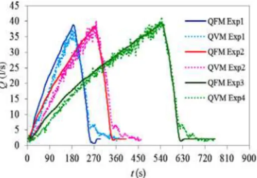
The discharge obtained from the electromagnetic flow meter mounted on the pipe is denoted as QFM.

The time variation of QFM and QVM are depicted in

Fig. 4.Time variation of the Q_FM and Q_VM. The total volume of water under the hydrograph Exp1 are 5.87 m3 and 5.55 m3 (5.4% difference) considering QFM (FM) and QVM (VM), respectively. The volume obtained in the pipe 14.34 m3 _{and in the flume is 13.93 m}3 _{(2.8% difference).} The average value for the ratio throughout the experiments is 1.059 for Exp1, 1.043 for Exp2 and 1.030 for Exp3. Therefore the measurements can be considered to be representing the discharge in the flume satisfying the continuity within the experimental system. This shows that the flow rate do not change too much for pipe flow and for open channel flow.

The flow depth variation with dimensionless time (t/Tr) at x= 9 m is given in Fig. 5. At the base flow,

before the hydrograph started, the water surface slope was determined by measuring the flow depth at various points and calculated as h/xbase = 0.0033. The variation of the water surface profile is given in Fig. 6.a and Fig. 6.b for Exp1 and Exp3, respectively. The profiles are given at times 0.0, 0.2, 0.4, 0.6, 0.8 and 1.0 times Tr of the rising

period. It is observed that the water depth at the downstream never becomes smaller than the upstream water depth for all phases of the hydrograph.

Fig. 5. Variation of flow depth h with t/Tr.

The characteristics of the experiments are given in Table 1. Here F _{base and} F _{peak are the Froude} numbers at base and peak flow conditions, respectively. The subscripts “VM” and “FM” corresponds to the parameter obtained considering QVM and QFM, respectively. Tr V is the rising

duration considering the velocity. As seen from the table, all experiments were conducted under

subcritical flow conditions.

Fig. 6. Water surface slopes at various times for (a) Exp1 and (b) Exp3.

5.

E

S

V

The methods given in the introduction part for calculating the shear velocity are adopted for the case in this study. Among them, the momentum equation (u*UN), the Saint-Venant method (u*SV),

Clauser Method (u*L) the Parabolic Law (u*P), and

(u*avg) are used. The velocity data in the viscous

sub-layer could not be measured since the boundary layer thickness 11.6/u* is very small, therefore this

method was not used. Also since the total shear stress does not obey the linear distribution any longer in unsteady flows, it is decided not to use the Reynolds Stress graph method. The shear velocities are calculated and discussed below.

5.1.

Shear Velocity Calculations

1. The Slope Method, Saint-Venant Equations (u*UN

& u*SV):

The velocity measurements were carried out only at one section i.e. 9 m from the channel entrance. Therefore it was not possible to calculate the term





magnitude 10-5 while the S0 or Se has an order of 10

-3 _{(Graf and Alt}

ınakar, 1998). It was assumed that the spatial variation of velocity in the channel is negligible (Powell et al. 2001, Hassan et al. 2006). Therefore the term





0 / 

Q x thus the shear velocity becomes,

    

  

          

 

  

t V g h V g x h S gR

u h

1 1 1 2 0

*

Fig. 7.The variation of h/x (V2_{/gh-1) term with}

normalized time t/Tr.

-0.00440 -0.00400 -0.00360 -0.00320 -0.00280 -0.00240

0 90 180 270 360 450 540 630 720 810

-

h/



x

t (s)

Exp1

Exp2

Exp3

0.00000 0.00004 0.00008 0.00012 0.00016

0 90 180 270 360 450 540 630 720 810

(



h/



x)

(

V

2/

gh

)

t (s)

Exp1

Exp2

Exp3

-0.00040 -0.00020 0.00000 0.00020 0.00040 0.00060

0 90 180 270 360 450 540 630 720 810

-(

1

/

g

)(



V/



t

)

t (s)

Exp1

Exp2

Exp3

(a)

(b)

(c)

Fig. 8. (a) second, (b) third and (c) fourth terms in Eq. (17) for experiments.

One can rewrite the Eq. (16) as Eq. (17). The time variation of the second, third and fourth terms in the parenthesis of Eq. (17) which are -h/x, (V2/gh)h/x and (1/g)V/t, respectively are given

in Fig. 8.a, 8.b and 8.c, respectively for the experiments. The minimum value of ∂h/∂x occurs at 250 s, 340 s and 620 s for Exp1, Exp2 and Exp3, respectively. The spatial-variation of the flow depth depends on the downstream boundary conditions of the flume. It is equal to 0.0034 for the leading and tailing steady flows, i.e. the steady parts preceding and proceeding the hydrograph. When the flow increases, the spatial-variations of the flow depth, h start to decrease till minimum values of 0.004 when the flow reaches its peak value. The spatial-variation of h went back to their steady state after fluctuating around it.

    

  

         

t V g x h h V g x h S gR

u h

1 1 2 0

*

The variation of the second term (V2/gh)(∂h/∂t) with time attains its peak value as 180 s, 270 s and 540 s for the hydrographs Exp1, Exp2 and Exp3, respectively. The third term –(1/g)(∂V/∂t) for Exp1 has more fluctuations in the rising limb when compared with those for Exp2 and Exp3. This is attributed again to the wave propagation in the flume. It is seen that the magnitude of the second and third terms are much less than spatial-variations. Obviously the spatial-variations have the dominating roles as mentioned by Qu (2002).

2. Clauser Method (u*L):

In this study the Clauser Method used by Cellino (1998) was adopted and modified for the unsteady flow case. The linear best fit line of u versus ln(z) was obtained for each velocity profile measured at each sampling time as performed by Qu (2002), Nezu and Sanjou (2006) and Tu (1991). The mean value of the correlation coefficients R2 for Exp1 was around 0.8 and for Exp2 and Exp3, it is 0.6.

3. Parabolic Law (u*P):

The correlation coefficient R2 is calculated as 0.6 for Exp1, 0.56 for Exp2 and 0.55 for Exp3, when the best fit line is drawn between u and (1-z/h)2. The

 is taken as 7.8 and the maximum velocity calculated from the u intercept. As depicted in Fig. 9, the um obtained from the measured velocity time

series is in accord with the calculated one for all experiments.

Fig. 9.um obtained from the measured velocity

4. Average Velocity (u*avg):

The Eq. (14) is used to find the shear velocity by using the mean average velocity V. The equivalent sand roughness was taken as ks = 10 d50.

5.2.

Comparison of the Results

The time variation of the obtained shear velocities named as u*UN, u*SV, u*L, u*P and u*avg are depicted

in Fig. 10.

Fig. 10.The variation of shear velocity u* with

time for (a) Exp1, (b) Exp2 and (c) Exp3.

The percentage deviations from the shear velocity found by Clauser method from the other shear velocities are calculated and the root mean square values are given in Table 2, for the rising, falling and total durations. Kironoto (1993) calculated the shear velocity by the Reynolds stress graph and Clauser Method. He found the greatest deviation from the shear velocity obtained by Clauser method is the one found by energy slope method. The percentage difference was in the range of ±20%. Qu (2002) calculated the shear velocity by Clauser method, slope method and in his conclusions in his study on sediment transport. Qu (2002) found that the shear velocity, u∗SV estimated from Saint-Venant

equations is smaller than the others. There is no one shear velocity whose root mean square (RMS) value is the lowest for all. Afzalimehr et al (2007) also mentioned that the parabolic law is applied when the data are far from the bed so as a reference the shear velocity calculated by the parabolic law is also considered and the deviations found by parabolic law are given in Table 3. Unlike the Clauser method, it is observed that the shear velocity calculated by average velocity equation has particularly the lowest RMS value. The critical shear velocity u*UN was overestimated due to the

steady and uniform flow assumption. The u*SV was

also overestimated particularly during the first phases of the hydrograph. On the other hand u*P and

u*avg coincides well. It is concluded that the shear

velocities found by the parabolic law and the average velocity equation can be used interchangeably.

Table 2 Deviation of the shear velocities from the one calculated by Clauser method

RMS (cm/s)

u*UN u*SV u*P u*avg

Rising 4.36 0.56 0.81 0.91 Exp1 Falling 5.39 0.93 0.49 0.53

Total 4.90 0.77 0.67 0.74

Rising 4.54 0.50 0.58 0.80 Exp2 Falling 5.18 0.81 0.68 0.65

Total 4.72 0.60 0.60 0.76

Rising 4.61 0.70 0.79 0.74 Exp3 Falling 5.51 1.00 0.36 0.22

Total 4.84 0.78 0.71 0.66

Table 3 Deviation of the shear velocities from the one calculated by parabolic law

RMS (cm/s)

u*UN u*SV u*P u*avg

Rising 5.00 0.55 0.81 0.35

Exp1 Falling 5.44 0.87 0.49 0.24

Total 5.23 0.73 0.67 0.30

Rising 5.03 0.60 0.39 0.34

Exp2 Falling 5.32 0.88 0.76 0.24

Total 5.18 0.76 0.60 0.29

Rising 5.26 0.92 0.79 0.21

Exp3 Falling 5.72 0.77 0.36 0.18

Total 5.37 0.89 0.71 0.20

5.3.

Velocity Profiles

The velocity profile measured and the velocity values obtained by logarithmic and parabolic laws are given in Fig. 11 at t/Tr equal to 0.3, 0.6 and 0.8

for the experiments. Here the solid line represents the best fit line obtained by logarithmic and parabolic laws. Kundu and Ghoshal (2012) also combined the logarithmic law for inner region and the parabolic law for outer region.

6.

H

velocity values are also given in the same figure. As it is expected the maximum velocity values at z=10.5 cm are all greater than the ones corresponding to the velocity values at z=2.5 cm. The ratios are 1.21, 1.18 and 1.13 for Exp1, Exp2 and Exp3, respectively. This reveals that the greater the unsteadiness the higher the maximum point velocity occurs close to the surface than close to the bottom.

0 2 4 6 8 10 12 14 16

0 10 20 30 40

z

(c

m

)

u(cm/s) Exp1

Exp1 Exp2 Exp2 Exp3 Exp3

0 2 4 6 8 10 12 14 16

0 10 20 30 40

z

(c

m

)

u(cm/s) Exp1

Exp1 Exp2 Exp2 Exp3 Exp3

0 2 4 6 8 10 12 14 16

0 10 20 30 40

z

(c

m

)

u(cm/s) Exp1

Exp1 Exp2 Exp2 Exp3 Exp3

(a)

(b)

(c)

Fig. 11. Velocity profiles for the experiments at for (a) t/Tr = 0.3, (b) t/Tr = 0.6 and (c) t/Tr = 0.8,

here the solid line represents the best fit line.

The clock-wise hysteresis is observed for both hydrographs given in Fig 12. The rising and falling limbs are close to each other for Exp3 in which the unsteadiness is small whereas for Exp1, the limbs become further apart. This distance between the limbs depends on the unsteadiness of the hydrograph as mentioned by Graf and Altınakar (1998).

A hysteresis intensity parameter  is proposed as given in equation below in order to calculate how far the limbs from each other. The area between the limbs is normalized by the unit discharge difference of corresponding to the peak and base values, qpeak

and qbase, respectively.

base peak n

i

i i i

q q

u h h

 











 ) /2

( 2

1

1 2



It is revealed that the hysteresis intensity parameter

 increases with flow depth, in other words the more you are close to the surface the hysteresis is felt more.

It may also be concluded that the constant of the power trend line curve drawn for Exp1 is greater than the one obtained for Exp2 which is also greater than Exp3. This means the more the unsteady the hydrograph the more the hysteresis .

Fig. 12.Variation of u with h (a) Exp1, (b) Exp2 and (c) Exp3.

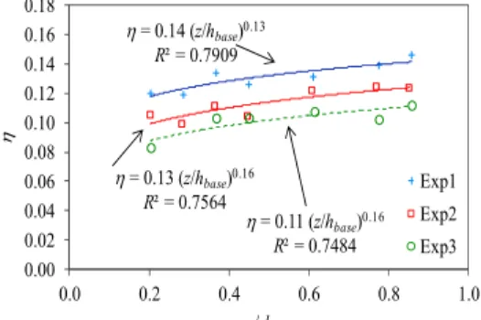
The variation of hysteresis intensity parameter  with normalized elevation as z/hbase, is depicted in

= 0.14 (z/hbase)0.13

R² = 0.7909

= 0.13 (z/hbase)0.16

R² = 0.7564

= 0.11 (z/hbase)0.16

R² = 0.7484 0.00

0.02 0.04 0.06 0.08 0.10 0.12 0.14 0.16 0.18

0.0 0.2 0.4 0.6 0.8 1.0



z/ hbase

Exp1 Exp2 Exp3

Fig. 13. The variation of  with z/hbase.

13 . 0 14 .

0 _

     

base h

z



16 . 0 13 .

0 _

     

base h

z



16 . 0 11 .

0 _

     

base h

z



The variation of cross sectional mean velocity V and flow depth h is given in Fig. 14. It is observed that when the unsteadiness is less as for Exp3, the rising and falling limbs are close to each other, whereas for Exp1, the limbs become further apart. When the mean average velocity Vi+1 is inserted for

ui+1 in Eq. (18), the hysteresis intensity parameter is

calculated as 0.12, 0.11 and 0.09 for Exp1, Exp2 and Exp3, respectively.

Fig. 14. The variation of velocity V with h.

7.

C

The shear velocity is an important parameter in characterizing the shear at the boundary and there exist methods to estimate the shear velocity in steady flows. These methods are listed as the use of the Saint-Venant equations u*SV, use of the

procedure given by Clauser Method u*L, use of the

parabolic law u*P, use of the momentum equation

assuming the slope of energy grade line is equal to bed slope u*UN and use of the average velocity

equation u*avg. The methods which are used to

calculate the shear velocity in steady flows were tested under unsteady flow conditions for three

asymmetrical triangular-shaped hydrographs.

The stream-wise and vertical components of velocity time series and the velocity profiles were obtained by means of an acoustic Doppler velocity meter. The instantaneous velocity time series were obtained at various vertical elevations and the moving average algorithm is adopted to obtain the time varying mean velocity. The variation of flow depth at various locations along the flume was used to calculate the water surface and energy slope variation. It is observed that the water depth at the downstream never becomes smaller than the upstream water depth which means a positive water surface slope throughout the flume for all phases of the hydrograph. Assuming the spatial variation of velocity in the channel is negligible, the Eq. (17) is obtained by which the u*SV can be calculated. It is

seen that the magnitude of the second ((V2/gh)h/x) and third ((1/g)V/t) terms are much less than spatial-variations. Obviously the spatial-variations (-h/x) have the dominating roles. The momentum equation assuming the flow is uniform was used to calculate the shear velocity u*UN.

The shear velocity was also calculated as u*L by

using the Clauser method. The shear velocity calculated by using the parabolic law as u*L and it is

observed that the maximum velocity um obtained from the measured velocity time series is in accord with the calculated one. The well-known average velocity equation was used to obtain the shear velocity as u*avg.

Among the methods, u*UN and particularly during

the first phases of the hydrograph u*SV were

overestimated. On the other hand u*P and u*avg

coincides well. It is concluded that the shear velocities found by the parabolic law and the average velocity equation can be used interchangeably.

The logarithmic law for inner region and the parabolic law for outer region combined in order to obtain the mean velocity profiles. Furthermore the hysteresis was investigated and a hysteresis intensity parameter is proposed in order to see the depth variation of hysteretic behavior at point velocity. It is revealed that the hysteresis intensity parameter  increases with flow depth, in other words the more you are close to the surface the hysteresis is felt more. The hysteresis parameter was adapted to the variation of cross-sectional mean velocity and flow depth. It is revealed that the more the unsteady the hydrograph the more the hysteresis both in terms of point velocity and cross-sectional mean velocity.

A

R

Abda, F., A. Azbaid, D. Ensminger, S. Fischer, P. François, P. Schmitt and A. Pallarés (2008) Ultrasonic device for real-time sewage velocity and suspended particles concentration measurements. 11th International Conference on Urban Drainage, ISUD, Edinburgh, Scotland, UK.

Absi, R. (2011) An ordinary differential equation for velocity distribution and dip-phenomenon in open channel flows. Journal of Hydraulic Research 49(1), 82–89.

Afzalimehr, H., S. Dey and P. Rasoulianfar (2007). Influence of decelerating flow on incipient motion of gravel-bed stream. Sadhana 32(5), 545-559.

Akhavan, R., R. D. Kamm and A. H. Shapiro (1991). An investigation of transition to turbulence in bounded oscillatory stokes flows. Journal of Fluid Mechanics 225, 395-422. Alabi, P. D. (2006). Time development of local

scour at a brı_{dge p}ı_{er f}ı_{tted w}ı_{th a collar,}

M.Sc. Thesis, University of Saskatchewan, Canada.

Bagherimiyab, F. (2012). Sediment suspension dynamics in turbulent unsteady, depth-varying open-channel flow over a gravel bed. PhD Thesis No: 5168, Ecole Polytechnique Fédérale (EPFL), Lausanne, Switzerland.

Bares, V., J. Jirak and J. Pollert (2008). Spatial and temporal variation of turbulence characterisitcs in combined sewer flow. Flow Measurement and Instrumentation 19(3-4), 145-154. Beheshti, A. A. and B. Ataie-Ashtiani (2010).

Experimental study of three-dimensional flow field around a complex bridge pier. Journal of Engineering Mechanics 136(2), 143-154. Bombar, G. (2014). Velocity time series obtained

around a bridge pier during a scour hole development. Proceedings of 3rd IAHR Europe Congress, Porto, Portugal.

Bombar, G., M. Ş. Güney, G. Tayfur and Ş. Elçi (2010). Calculation of the time-varying mean velocity by different methods and determination of the turbulence intensities. Scientific Research and Essays 5(6), 572-581. Bombar, G., Ş. Elçi, G. Tayfur, M. Ş. Güney and A.

Bor (2011). Experimental and numerical investigation of bedload transport under unsteady flows. Journal of Hydraulic Engineering 137(20), 1276-1282.

Bonakdari, H., F. Larrarte, L. Lassabatere and C. Joannis (2008). Turbulent velocity profile in fully-developed open channel flows. Environmental Fluid Mechanics 8(1), 1–17. Bose, S. K. and S. Dey (2012). Turbulent unsteady

flow profiles over an adverse slope, Acta Geophysica 61(1), 84-97.

Brereton, G. J. and R. R. Mankbadi (1995). Review of recent advances in the study of unsteady turbulent internal flows. Applied Mech. Rev. 48(4), 189-212.

Brereton, G. J., W. C. Reynolds and R. Jayaraman (1990). Response of a turbulent boundary layer to sinusoidal free-stream unsteadiness. Journal of Fluid Mechanics 221, 131-159.

Cardoso, A. H., W. H. Graf and G. Gust (1989). Uniform flow in a smooth open channel. Journal of Hydraulic Research 27(5), 603-616. Cellino, M. (1998). Experimental study of

suspension flow in open channels, PhD Thesis, No. 1824, Ecole Polytechnique Fédérale (EPFL), Lausanne, Switzerland.

Coles, D. (1956). The law of the wake in the turbulent boundary layer, Journal of Fluid Mechanics 1(2), 191-226.

Cui, H. and V. P. Singh (2013) Two-dimensional velocity distribution in open channels using Tsallis Entropy. Journal of Hydraulic Engineering 18(3), 331–339.

Cui, H. and V. P. Singh (2014) Computation of suspended sediment discharge in open channels by combining Tsallis Entropy-based methods and emprical formulas. Journal of Hydraulic Engineering 19(1), 18–25.

Cui, H. and V. P. Singh (2014) One-dimensional velocity distribution in open channels using Tsallis Entropy. Journal of Hydraulic Engineering 19(2), 290–298.

Cui, H. and V. P. Singh (2014) Suspended sediment concentration in open channels using Tsallis Entropy. Journal of Hydraulic Engineering 19(5), 966–977.

Debnath, R., A. Mandal, S. Majumder, S. Bhattacharjee and D. Roy (2015). Numerical analysis of turbulent fluid flow and heat transfer in a rectangular elbow. Journal of Applied Fluid Mechanics 8(2), 231–241. FlowTracker Handheld ADV User’s Manual

Firmware Version 3.1 SonTek/YSI, Inc., 2006.

Genç, O., M. Ardıçlıoğlu and N. Ağıralioğlu (2015). Calculation of mean velocity and discharge using water surface velocity in small

streams. Flow Measurement and

Instrumentation, online publication date: 1-Mar-2015.

Graf, W. H. and M. S. Altınakar (1998). Fluvial Hydraulics, John Wiley & Sons Inc.

Griffiths, G. A. (1981). Flow resistance in coarse gravel bed rivers. Journal of the Hydraulics Division 107(7), 899-918.

Guo, J. (2014). Modified log-wake-law for smooth rectangular open channel flow. Journal of Hydraulic Research 52(1), 121–128.

Guo, J. and P. Y. Julien (2003). Modified log-wake law for turbulent flows in smooth pipes. Journal of Hydraulic Research 41(5), 493– 501.

Guo, J. and P. Y. Julien (2008). Application of the modified log-wake law in open-channels. Journal of Applied Fluid Mechanics 1(2), 17– 23.

Guo, J., P. Y. Julien and R. N. Meroney (2005). Modified log-wake law for zero-pressure-gradient turbulent boundary layers. Journal of Hydraulic Research 43(4), 421–430.

Hassan, M. A., R. Egozi and G. Parker (2006). Experiments on the effect of hydrograph characteristics on vertical grain sorting in gravel bed rivers. Water Resources Research (42), 1-15.

Jan, C. D., J. S. Wang and T. H. Chen (2006). Discussion of Simulation of flow and mass dispersion in meandering channel. Journal of Hydraulic Engineering 132(3), 339-342. Jensen, B., B. M. Sumer and J. Fredsoe (1989).

Turbulent oscillatory boundary layers at high Reynolds numbers. Journal of Fluid Mechanics 206, 265-297.

Kabiri-Samani, A., F. Farshi and M. R. Chamani (2013). Boundary shear stress in smooth trapezoidal open channel flows. Journal of Hydraulic Engineering 139(2), 205–212. Kırkgöz, S. (1989). Turbulent velocity profiles for

smooth and rough open channel flow. Journal of Hydraulic Engineering 115(11), 1543-1561. Kırkgöz, S. and M. Ardıçlıoğlu (1997). Velocity

profiles of developing and developed open channel flow. Journal of Hydraulic Engineering 123(12), 1099–1105.

Kironoto, B. A. (1993). Turbulence characteristics of uniform and non-uniform, rough open-channel flow. Ph.D.Thesis, No 1094, Ecole Polytechnique Fédérale (EPFL), Lausanne, Switzerland.

Kumar, P., A. Mishra, N. S. Raghuwanshi and R. Singh (2002). Application of unsteady flow hydraulic-model to a large and complex irrigation system. Agricultural Water Management 54, 49-66.

Kundu, S, and K. Ghoshal (2012). Velocity distribution in open channels: combination of log-law and parabolic-law. World Academy of Science, Engineering and Technology 68, 2151-2158.

Larrarte, F. and E. Le Barbu (2010). Acoustic profilers and pollutant flux measurements in urban hydrology NOVATECH Session 2.4.

Lassabatere, L., J. Pu, H. Bonakdari, C. Joannis and

F. Larrarte (2013). Velocity distribution in open channel flows: analytical approach for the outer region. Journal of Hydraulic Engineering 139(1), 37–43.

Leopold, L. B., M. G. Wolman and P. Miller (1964). Fluvial Processes in Geomorphology, W.H. Freeman and Company 522.

Lhermitte, R. and U. Lemmin (1994). Open-channel flow and turbulent measurement by high-resolution Doppler sonar. Journal Atmos. Oceanic Technol. 11(5), 1295-1308

Liu, Z. (2001). Sediement transport, Laboratoriet for Hydraulik og Havnebygning, Instituttet for Vand, Jord og Miljøteknik, Aalborg Universitet.

Lopez, F. and M. H. Garcia (1999). Wall similarity in turbulent open-channel flow. Journal of Hydraulic Engineering 125(7), 789-796. Meselhe, E. A. and F. M. Holly (1993). Simulation

of unsteady flow in irrigation canals with dry bed. Journal of Hydraulic Engineering 119(9), 1021-1039.

Muste, M. and V. C. Patel (1997). Velocity profiles for particles and liquid in open-channel flow with suspended solids. Journal of Hydraulic Engineering 123(9), 742-751.

Nezu, I. (2005). Open-channel flow turbulence and its research prospect in the 21st century. Journal of Hydraulic Engineering 131(4), 229-246.

Nezu, I. and H. Nakagawa (1993). Turbulence in open-channel flows, IAHR Monograph Series, A. A. Balkema Publishers, Rotterdam, The Netherlands

Nezu, I. and M. Sanjou (2006). Numerical calculation of turbulence structure in depth-varying unsteady open-channel flows. Journal of Hydraulic Engineering 132(7), 681-695. Nezu, I. and W. Rodi (1986). Open channel flow

measurements with a laser Doppler anemometer. Journal of Hydraulic Engineering 112(5), 335-355.

Nezu, I., A. Kadota and H. Nakagawa (1997). Turbulent structure in unsteady depth-varying open-channel flows. Journal of Hydraulic Engineering 123(9), 752–763.

Nezu, I., and H. Nakagawa (1991). Turbulent structures over dunes and its role on suspended sediments in steady and unsteady open-channel flows. Proc. of Int. Symp. on Transport of Suspended Sediments and its Mathematical Modeling, IAHR, Firenze 165-189.

Nikuradse, J. (1933). Laws of flow in rough pipes, Translation in National Advisory Committee for aeronautics, technical memorandum 1292, NACA, Washington 1950, 62.

unsteady open-channel flows. D1-Turbulent Channel Flows with Macro Roughness Vegetation. 28th Congress of IAHR, Graz, Austria, Conf. Proceedings.

Patel, P. L. and K. G. Ranga Raju (1999). Critical tractive stress of nonuniform sediments. Journal of Hydraulic Research 37(1), 39–58. Powell, D. M., I. Reid and J. B. Laronne (2001).

Evolution of bed load grain size distribution with increasing flow strength and the effect of flow duration on the caliber of bed load sediment yield in ephemeral gravel bed rivers. Water Resources Research 37(5), 1463-1474. Qu, Z. (2002). Unsteady open-channel flow over a

mobile bed. Ph.D. Thesis. No 2688, Ecole Polytechnique Fédérale (EPFL), Lausanne, Switzerland.

Rowınski, P. M., W. Czernuszenko and J. M. Pretre (2000). Time-dependent shear velocities in channel routing. Hydrological Sciences 45(6), 881-895.

Shah S. A., A. C. Orifici and J. H. Watmuff (2015). Water impact of rigid wedges in two-dimensonal fluid flow. Journal of Applied Fluid Mechanics 8(2), 329-338.

Singh V. P., A. Byrd and H. Cui (2014). Flow duration curve using entrophy theory. Journal of Hydraulic Engineering 19(7), 1340-1348. Song, C. G., I. W. Seo and Y. D. Kim (2012).

Analysis of secondary current effect in the modeling of shallow flow in open channels. Advances in Water Resources 41, 29-48. Song, T. (1994). Velocity and turbulence

distribution in non-uniform and unsteady openchannel flow. Ph.D. Thesis, No. 1324,

Ecole Polytechnique Fédérale (EPFL), Lausanne, Switzerland.

Song, T. and W. H. Graf (1996). Velocity and turbulence distribution in unsteady open channel flows. Journal of Hydraulic Engineering 122(3), 141-154.

Tardu, S. F, G. Binder and R. F. Blackwelder. (1994). Turbulent channel flow with large-amplitude velocity oscillations. Journal of Fluid Mechanics 267, 109-151.

Tu, H. (1991). Velocity distribution in unsteady flow over gravel beds. Ph.D. Thesis, No 911, Ecole Polytechnique Fédérale (EPFL), Lausanne, Switzerland.

Tu, H. and W. H. Graf (1992). Velocity distribution in unsteady open channel flow over gravel beds. Journal of Hydroscience and Hydraulic Engineering 10(1), 11-25.

Walker, W. R. and A. S. Humpherys (1983). Kinematic-wave furrow irrigation model. Journal of Drainage and Irrigation Engineering 109(4), 377–392.

Wiberg, P. L. and J. D. Smith (1987). Calculations of the critical shear stress for motion of uniform and heterogeneous sediments. Water Resouces Research 23(8), 1471–1480. Yang, S. Q. (2010). Depth-averaged shear stress

and velocity in open-channel flows. Journal of Hydraulic Engineering 136(11), 952–958. Zhang, S., J. G. Duan, T. S. Strelkoff and E.