ON THE EFFICIENCY OF RELATIONAL,
DOCUMENT AND GRAPH DATA MODELS FOR
PEDRO ONOFRE SANTOS
EFICIÊNCIA DOS MODELOS DE DADOS
RELACIONAL, DOCUMENTO E GRAFO PARA O
GERENCIAMENTO DE DADOS GEOGRÁFICOS
MÓVEIS
Dissertação apresentada ao Programa de Pós-Graduação em Ciência da Computação do Instituto de Ciências Exatas da Univer-sidade Federal de Minas Gerais como req-uisito parcial para a obtenção do grau de Mestre em Ciência da Computação.
Orientador: Mirella Moura Moro
Coorientador: Clodoveu Augusto Davis Jr.
Belo Horizonte
PEDRO ONOFRE SANTOS
ON THE EFFICIENCY OF RELATIONAL,
DOCUMENT AND GRAPH DATA MODELS FOR
MANAGING MOBILE SPATIAL DATA
Dissertation presented to the Graduate Program in Computer Science of the Fed-eral University of Minas Gerais in partial fulfillment of the requirements for the de-gree of Master in Computer Science.
Advisor: Mirella Moura Moro
Co-Advisor: Clodoveu Augusto Davis Jr.
Belo Horizonte
c
2015, Pedro Onofre Santos. Todos os direitos reservados.
Santos, Pedro Onofre
S237e On the efficiency of relational, document and graph data models for managing mobile spatial data / Pedro Onofre Santos. — Belo Horizonte, 2015
xxii, 72 f. : il. ; 29cm
Dissertação (mestrado) — Universidade Federal de Minas Gerais – Departamento de Ciência da
Computação.
Orientadora: Mirella Moura Moro
Coorientador: Clodoveu Augusto Davis Jr.
1. Computação – Teses 2. Benchmarking
(Administração) - Teses. 3. Avaliação de desempenho – Teses. 4. Sistemas de informação geográfica – Teses. I. Orientadora. II. Coorientador. III. Título.
Acknowledgments
My most sincere thanks to Mirella and Clodoveu for their knowledge, guidance, patience and willingness to help me in any way. This work wouldn’t be nearly as possible without them.
I also want to thank Ruth for her kindness, understanding, patience and support, she is the best person in the world.
My thanks to the peers and colleagues which helped so much during my studies: Bruno dos Santos Azevedo Cardoso, Cássia do Carmo Vieira, Tarcísio Guerra Savino Filó, Harlley Augusto de Lima, Daniel Hasan Dalip, Keiller Nogueira, Rodrigo Augusto da Silva Alves and Wladston Viana Ferreira Filho.
Also, I want to thank all my old Eletra’s friends, whose friendship endured for the last ten years: Amanda, Burns, Cabeça, Cuia, Denis, Denise, Emo, Hudson, Jana, Junca, Luiz, Lula, Madruga, Pardal, Peão, Rafa, Sabará, Samsam, Sidoca, Sir and Thi. In that list, not mutually exclusive, but I want to thank our Dota 2 buddies which helped our stress levels rise and our win rate fall: Bill, Brunasso, Cuia, Daleste, Giuli, Jovem, Lula, Palhaço, Pardal, Sabará, Sir, Tutor and Vjunca.
I also want to thank my parents for letting me live rent free for 25 years and my grandmas for the much needed meals and desserts. If I have forgotten your name, know that this work would not be possible without all the people in my life, as they are too many to remember, I’m sorry.
Lastly, I want to thank God who has always been there for me.
This work is supported by a FAPEMIG scholarship. This financial support is gratefully acknowledged.
“What is better - to be born good, or to overcome your evil nature through great effort?” (Paarthurnax)
Resumo
Vários dos sistemas de informação atuais apresentam volume de dados crescente com-binado com diversidade e mobilidade de suas aplicações. Entretanto, selecionar uma infraestrutura computacional apropriada é ainda um grande desafio para projetistas de tais sistemas. Esta dissertação demonstra como técnicas de avaliação de desempenho atuais podem não ser ideais para comparar o desempenho de sistemas de bancos de dados espaciais. Particularmente, considera-se as necessidades de usuários móveis, as quais incluem tráfego constante de dados espaciais, tais como consulta por pontos de interesse, visualização de mapas, zoom e caminhamento, roteamento e rastreamento de localização. A avaliação realizada mostra que para obter uma comparação justa é necessário utilizar cargas específicas (de dados e consultas) para cada característica móvel - o que não é atualmente obtido através das ferramentas de benchmark presen-tes no mercado. São também comparadas tecnologias de sistemas de dados relacionais, orientados a documentos e baseados em grafos (NoSQL). De modo geral, este estudo demonstra que as metodologias genéricas de benchmark não são ótimas e podem levar a um projeto físico longe do ideal.
Palavras-chave: Análise de Desempenho, Bancos de Dados Geográficos, NoSQL, Big Data.
Abstract
Increasing data volume, application diversity and mobility are the foremost character-istics of many current information systems. However, selecting the appropriate compu-tational infrastructure is still a hard task for the designers of such systems. This work demonstrates how current performance evaluation techniques may not be ideal when comparing the performance of spatial database management systems. Specifically, we consider the needs of mobile users that involve constant spatial data traffic, such as querying for points of interest, map visualization, zooming and panning, routing and location tracking. Our evaluation shows that a fair comparison requires specific work-loads for each mobile feature – which is not currently achievable by the industry’s stan-dard benchmark tools. We then compare technologies in relational (SQL), document-oriented and graph-based DBMSs (NoSQL). Overall, this study demonstrates that the one-size-fits-all benchmark methodologies are not optimal and may lead to a far from an ideal system design.
Keywords: Benchmark, Spatial Databases, NoSQL, Big Data.
List of Figures
1.1 Brazilian main highways in blue with a spatial buffer for BR-040 highlighted. 2
1.2 Nearby points of interest searched by the user. . . 3
2.1 Katrina’s area of effect, the size of the circle and coloration represent the hurricane’s speed. . . 8
2.2 OMT-G schema fragment for user position tracking. . . 9
2.3 User position tracking in a relational DBMS table. . . 10
2.4 User position tracking document. . . 10
2.5 User position tracking graph. . . 11
2.6 Multiple raster images of North America as a background map1. . . . 12
2.7 Vector data of the Brazilian states with Minas Gerais highlighted. . . 13
2.8 Roads (linestrings) and intersections (points) as vector data. . . 14
2.9 The same objects from Figure 2.8 now mapped into a traversable network. 14 2.10 Spatio-temporal raster data monitoring the deforestation process in Itaúba, MT, Brazil, from 1990 to 2007. . . 15
2.11 User’s location history recorded by Google Maps. . . 16
3.1 Outskirts of Hong Kong. . . 23
3.2 R-tree example, minimum bounding rectangles over space and the respective tree structure. . . 26
3.3 Continental USA states’ bounding boxes. . . 27
3.4 Continental USA states’ Geohash space-filling curve combination. . . 28
3.5 Z curve distance example. . . 28
4.1 2013 TIGER/Line collections AREALM, AREAWATER, ROADS, PRISE-CROADS, PRIMARYROADS and POINTLM at the Manhattan’s Central Park. . . 32
4.2 DE-9IM over spatial object interactions. . . 35
4.3 TIGER Line OMT-G main classes diagram. . . 36
4.4 Thread schematic comparing Mongoimport with the new proposed solution. 40
4.5 Example of nearby POI within radius and equivalent PostgreSQL query. . 42
4.6 Example of nearby POI KNN and equivalent PostgreSQL query. The red mark is the device’s position and the blue marked locations are the possible answers. . . 42
4.7 Example of map view and equivalent PostgreSQL query. The user’s position is represented in red and the loaded results are highlighted within a rectangle for the “Area loaded”. . . 43
4.8 Example of calculated shortest path between points A and B and equivalent PostgreSQL query. . . 44
4.9 Recorded position history on the map and equivalent position insertion in PostgreSQL. . . 45
5.1 Distribution of query execution results (v/s). . . 52
5.2 Distribution of query execution results (v/s). . . 53
5.3 Distribution of query execution results (v/s). . . 54
5.4 Results for average vertices inserted per second. . . 55
5.5 Relative performance summary. . . 56
5.6 Neo4j JavaVM CPU Sampling. . . 57
A.1 Results for nearby POI within radius, percentile distribution. . . 69
A.2 Results for nearby POI k-NN, percentile distribution. . . 70
A.3 Results for map visualization, percentile distribution. . . 70
A.4 Results for map zooming, percentile distribution. . . 71
A.5 Results for map panning, percentile distribution. . . 71
A.6 Results for urban routing, percentile distribution. . . 72
A.7 Results for position tracking, percentile distribution. . . 72
List of Tables
1.1 Comparison between this study and previous related work. . . 4
3.1 Spatial metadata obtained from Figure 3.1. . . 23
3.2 DBMS Comparison. . . 24
4.1 DBMS Warm Up time. . . 30
4.2 2013 TIGER/Line vector collections. . . 33
4.3 Dataset disk consumption after data loading. . . 39
4.4 Dataset file import time for the original and implemented tools. . . 39
4.5 The main features, the spatial data type returned and what the evaluation measures for each query group. . . 41
5.1 Number of query executions per query set. . . 48
5.2 Evaluation parameters. . . 49
Contents
Acknowledgments ix
Resumo xiii
Abstract xv
List of Figures xvii
List of Tables xix
1 Introduction 1
2 Background and Related Work 7
2.1 NoSQL . . . 7
2.2 Spatial Data Models . . . 12
2.3 Big Data . . . 16
2.4 Spatial Big Data . . . 17
2.5 Discussion on Related Work . . . 17
3 Spatial DBMS 21 3.1 Mobile Systems . . . 21
3.2 DBMS Main Features . . . 23
3.3 Spatial Indexing . . . 25
4 Comparison Methodology 29 4.1 Processing Stages . . . 29
4.2 Dataset . . . 31
4.3 Data Modeling . . . 34
4.3.1 OMT-G . . . 35
4.3.2 Mapping Spatial Objects . . . 36
4.3.3 Graph Mapping for Urban Routing . . . 37 4.4 Data Loading . . . 38 4.5 Improvements on Data Loading . . . 39 4.5.1 Improving Mongoimport . . . 39 4.5.2 Improving Neo4j Load Strategy . . . 40 4.6 Spatial Queries . . . 41
5 Experimental Evaluation 47
5.1 Experimental Setup . . . 47 5.2 Parameters and Pre-evaluation . . . 48 5.3 Evaluation Metrics . . . 50 5.4 Performance Evaluation . . . 51 5.4.1 Nearby Points of Interest Within Radius and k-NN . . . 51 5.4.2 Urban Routing . . . 52 5.4.3 Map View . . . 52 5.4.4 Position Tracking . . . 54 5.5 Relative Performance Summary . . . 55
6 Conclusion 59
6.1 Summary of Contributions . . . 60 6.2 Future Work . . . 60
Bibliography 63
A Detailed Experimental Evaluation 69
Chapter 1
Introduction
The gathering and storage of spatial data regarding mineral resources, properties, wa-ter sources and other landscape attributes were always important tasks of organized human societies [14]. This however has changed greatly with the advance of computer systems capable of handling such data, which was previously limited to paper-written documents and maps. Such computer systems capable of processing and storing spatial attributes are called Geographic Information Systems (GIS). Traditional examples of GIS include: GRASS GIS1, QGIS2 and ArcGIS3.
Geographic information systems that provide public services often manage very large databases with lots of user requests. Such GIS applications require continuous availability, low response time and high throughput. Also, the underlying geographic databases deal with spatial objects with varying complexity, for which operations are much more expensive than in relational database management systems (RDBMS) that manage conventional data [15, 22, 32, 49, 51].
Specifically, the demand for GIS and spatially-enhanced applications, mostly for mobile devices, has increased alongside the user base. For example, in Brazil, the number of mobile devices grows rapidly and, according to the Brazilian Institute of Geography and Statistics (IBGE)4, it now reaches over 75% of the Brazilian population.
Such behavior reflects a pattern already present in the United States and Europe, making DBMS development a continuous task in order to excel upcoming challenges5.
1
GRASS GIS:http://grass.osgeo.org/
2
QGIS project: http://www.qgis.org
3 ArcGIS:http://www.arcgis.com/ 4 IBGE:http://www.ibge.gov.br/home/estatistica/pesquisas/pesquisa_resultados.php? id_pesquisa=40 5
MobiThinking Compendium of Mobile Statistics: http://mobiforge.com/research- analysis/global-mobile-statistics-2014-home-all-latest-stats-mobile-web-apps-marketing-advertising-subscriber
2 Chapter 1. Introduction
Figure 1.1: Brazilian main highways in blue with a spatial buffer for BR-040 high-lighted.
In this context, geographic location resources such as integrated Global Positioning System (GPS) modules made spatially-aware applications more attractive and useful. At the same time, such applications are more frequently used, reaching a point where most features accessed by the user contain geographic data and metadata.
Examples of spatially enhanced applications and geographic information systems in which geographic data is uploaded along with conventional data and metadata in-clude Google Maps6, Foursquare7and Waze8. The spatial abilities of those applications
make them so useful for so many people that a multi billion-dollar industry has been formed around them. Hence, the application’s performance, reliability and scalability play very important roles in the user’s decision to acquire and use such tools in a daily routine.
From the perspective of design and development of the databases underlying such applications, new requirements are becoming important. The trend towards novel management tools and techniques that replace Relational DBMS reflects such require-ments, particularly for big data [48]. However, it is still not clear how to select an adequate spatial data management tool, considering the requirements of current ap-plications, specially mobile ones. Such decision is far from simple, as current work shows incredible differences on evaluating queries over general and spatial big data (e.g., [21, 36, 49, 51] among many others).
6
Google Maps: http://maps.google.com
7
Foursquare: http://www.foursquare.com
8
3
Figure 1.2: Nearby points of interest searched by the user.
Spatial data is a multidimensional, more complex structure with slower processing time than primitive data types, such as bit, byte, integer, float as well as string, date and many others that are implemented in most DBMS. In a relational database, querying for data in a single table is straightforward in terms of query planning and hardware resource allocation. On the other hand, when performing spatial functions (mainly spatial joins), large amounts of memory are requested by the query, much more than the usual number/string processing, which leads to a large volume of allocated memory. Furthermore, the density of spatial objects on the dataset, the size of each object and even their shape can influence in the query performance.
For example, Figure 1.1 presents a map with Brazilian highways and highlights a spatial buffer created around highways Presidente Juscelino Kubitschek and Washing-ton Luís. These two highways form BR-040, which connects Brazil’s capital Brasília (DF) to Rio de Janeiro (RJ), one of the heaviest traffic highways in Brazil.
The density of spatial objects also plays an important role, as the queries for the nearby points of interest rely heavily on CPU processing power, alongside with the efficiency of spatial indexes. Figure 1.2 illustrates the result of a query for points of interest located near the user’s position in the center of the map.
4 Chapter 1. Introduction
Table 1.1: Comparison between this study and previous related work.
Study SQL NoSQL Real Workload Spatial Data Big Data
Spatial Star Schema Benchmark [40] ✓ ? ✕ ✓ ✕
TPC-C [10] ✓ ✕ ✕ ✕ ✕
BigBench [19] ✓ ✕ ✕ ✕ ✓
Jackpine [43] ✓ ✕ ✓ ✓ ✕
Our study ✓ ✓ ✓ ✓ ✓
More over, our evaluation differs from other studies in three crucial ways. First, we consider an interface where SQL and NoSQL data can be equally tested (even though with different designs, features and goals). Second, we propose a new metric (vertices per second) that is more tailored for evaluating mobile queries over spatial big data of varying complexity. This way, we are able to measure the DBMS efficiency towards geometric attributes, instead of only measuring how fast it processes a query. Third, we provide means to compare graph-based features obtained from spatial data. Nowadays, such features are very common in large systems, but they are usually treated by two separate models (network and spatial data). Table 1.1 is a summary of the points this study tackles compared to others.
Chapter 2 describes related work and background concepts in order to fully un-derstand spatial features. We also provide information about big data, non-relational models and DBMSs.
In Chapter 3, we present the spatial data mobile application scenario that is the base for this work. We also compare the main features of the three DBMSs considered in our evaluation. The spatial indexing features, as well as clustering and data distribution are further detailed, as they will have great impact on the performance analysis.
Chapter 4 introduces our methodology by explaining each processing stage, the dataset, the modeling characteristics and queries performed. Such discussion is impor-tant in order to demonstrate how a DBMS’s performance may vary only by changing the conceptual to logical mapping applied to its dataset. Note that current DBMS benchmark methodologies focus on synthetic data generators and parameter variations to simulate real world usage – as the industry’s standard TPC-H [42]. Here, the pro-posed workloads consider queries that reflect real operations performed by users of spatial mobile applications. We also provide alternatives to the data import tools for two of the tested DBMS.
capa-5
bilities9: PostgreSQL10with PostGIS11, MongoDB12, and Neo4j13with Neo4j-Spatial14.
Our evaluation results show that performance varies greatly in terms of algorithms and overall computational complexity due to each systems’ design. Therefore, selecting a spatial DBMS heavily depends on how well it handles the targeted spatial data and the most usual functions that the system is expected to perform.
Overall, by generating a workload that mimics real data, creating and experi-mentally evaluating a set of queries based on mobile systems’ features, this dissertation demonstrate that comparing spatial models and DBMSs requires new evaluation met-rics and methodologies. The main outcome of this dissertation includes demonstrating how performance evaluation should be data and system-oriented, based on the systems’ features and characteristics.
9
Using other DBMS requires adapting the database model and queries employed in our method-ology, which should be straightforward.
10
PostgreSQL:http://www.postgresql.org/
11
PostGIS: http://postgis.net/
12
MongoDB:http://www.mongodb.org/
13
Neo4j: http://www.neo4j.org/
14
Chapter 2
Background and Related Work
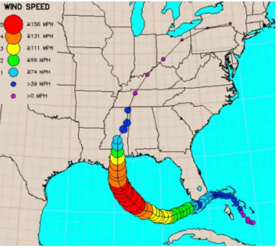
GIS and location-aware applications are becoming more common, sophisticated and necessary as user-based information increasingly becomes critical to all kinds of busi-nesses. Examples include location-based advertising, customer trace data, nearby points of interest, shortest routes and recommendation systems. Governments also seek spatial computing to obtain information about events and natural disasters. As an example, Figure 2.1 depicts the area affected by hurricane Katrina in 2005.
According to Shekhar et al. [48], processing spatial objects is more complex than classical computing, as they include geometric components (points, lines, polygons and variations) with a variable number of vertices. Moreover, the volume of data processed by applications like Google Maps or Waze easily surpasses the previous generation of spatial data “heavy lifters”, such as NASA’s Earth Observing System and other satellite imagery programs. Those applications (Google Maps in particular) already rely on NoSQL solutions to provide their users with more spatial features and faster spatial data querying [9, 22].
Next, we explain fundamental concepts regarding both NoSQL DBMS and spatial data. We also review previous related work, show how they implemented some features and techniques regarding spatial data, big data, benchmarking, and emphasize points that were not explored in comparison with our experimental evaluation.
2.1
NoSQL
NoSQL (often interpreted as Not Only SQL) is a class of database systems that are not necessarily relational in their structure and properties. Although non relational databases have been around since the late 1960s, only recently they have conquered mass market attention [34]. Specifically, NoSQL emerged in the last decade as an
8 Chapter 2. Background and Related Work
Figure 2.1: Katrina’s area of effect, the size of the circle and coloration represent the hurricane’s speed1.
ternative to horizontal and scalable data growth, aiming at improving the performance of RDBMS. According to Cattel [8], the main characteristics of those systems include: horizontal scaling among machine clusters, replicability and redundancy, simple in-terfaces and access protocols, heterogeneous ACID (Atomicity, Consistency, Isolation, Durability) controls (while some systems maintain full ACID support, others imple-ment only durability for example), efficient index distribution and memory usage, and dynamic attribute updates.
Over the past decade, industry has moved to a data-driven economy by requiring alternative data processing tools, mostly because RDBMS present issues when handling larger datasets. Large-scale systems have also moved from the relational environment to NoSQL [8, 18, 22, 34]. Such change increases the DBMS horizontal scalability, the ability to replicate themselves as well as index and memory efficiency. Nonetheless, NoSQL solutions also deal with weaker concurrency models by leaving some of the
1
2.1. NoSQL 9
Figure 2.2: OMT-G schema fragment for user position tracking.
ACID properties for the application layer to handle [26].
Furthermore, NoSQL systems rely on already consolidated simple query languages used in other data models (such as XML2 and JSON3) as a compact and efficient
way of specifying their queries while maintaining compatibility among heterogeneous operational and storage systems. They also benefit from performance and usability improvements on those models and their languages [7, 20, 39, 52, 54].
Overall, NoSQL Database Management Systems are the preferred choice when performance is a priority but consistency and concurrency restrictions are not very relevant, as in applications that require lots of data retrieval with little or no updating. Such choice is even more apparent as the volume of information handled by spatial DBMSs moves towards the realm of Big Data.
Relational DBMS are challenged by two main types of NoSQL DBMS. The first is the document-oriented model (for example, MongoDB), which has already absorbed most data from the Web 2.0 applications, previously based in RDBMS [18]. The second is the Business Intelligence, Digital Libraries and Analytical Systems type, in which relational data users have moved to solutions with higher processing power, such as those based on Apache Hadoop4.
Different NoSQL DBMS model and store data in heterogeneous ways. For exam-ple, consider an application where the user’s location history must be stored in order to reduce their commute time. It searches for an alternate route, in order to avoid heavy traffic, or it suggests optimal speeds in order to avoid red traffic lights. Such an application requires the simplest association between a user class and a location class. Such data definition is represented by the OMT-G [6] model as designed in Figure 2.2. Then, in order to emphasize each model’s unique features, the following figures repre-sent the same data using other data models: Figure 2.3 for relational tables, Figure 2.4 for document-oriented model, and Figure 2.5 for a graph-oriented model. Next, we go over some of the main features of those data models.
2
eXtensible Markup Language: http://www.w3.org/TR/REC-xml/
3
JavaScript Object Notation: http://json.org/
4
10 Chapter 2. Background and Related Work
Figure 2.3: User position tracking in a relational DBMS table.
Figure 2.4: User position tracking document.
• First, Codd [12] introduced the Relational Model. At the time it emerged, it surpassed many other systems with the advantage of removing from the users the necessity of knowing how data is stored in the machine. It presents data as relations or collections of tables, which are based on rows and columns, and provides operators to manipulate data stored in a tabular format. It also provides a service based on actions such as queries and data modification operators, which enables the user to retrieve and store data efficiently. The relational DBMS were the most important systems since Codd’s definition, turning file systems and other rudimentary database management systems obsolete.
2.1. NoSQL 11
Figure 2.5: User position tracking graph.
are usually represented by a language that provides either human readability or machine attribute mapping association, or both, such as XML, JSON and YML5.
• Graph-Oriented database management systems handle graph-like structures by associating data properties within nodes and relationships. The graph model enables querying a database based on a relationship attribute, which requires mul-tiple inner joins in a traditional relational DBMS. Consequently, Graph-Oriented DBMS are usually faster for associative data, which may grow immensely larger with the popularization of online social networks. The graph-oriented database model, as pointed out by Gyssens et al. [24], allows the representation and ma-nipulation of objects with a graph-based nature, which were previously modeled as the multi-join table sequence in the relational model.
Such a variety of choices poses challenges to system architects and their ability to stick with only one DBMS/data model. Usually one model will handle a set of queries better than the other. Finally, each model has its own challenges, as discussed in Section 4.3.
5
12 Chapter 2. Background and Related Work
Figure 2.6: Multiple raster images of North America as a background map6.
2.2
Spatial Data Models
There are four main models used to physically represent spatial data: raster, vector, network and spatio-temporal [47, 48]. Therastermodel uses a matrix of cells organized in rows and columns where each cell contains one or more pixels associated with an alpha-numeric value. Raster objects usually store visual, thermal and electromagnetic information obtained through aerial photographs, map scanning and satellite imagery. The information obtained is digitized and processed to provide detailed information about the targeted area. Raster data is often used as maps and map backgrounds for other GIS services. Figure 2.6 gives an example of raster data.
The vector model represents spatial objects as lists of vertex coordinates, thus configuring spatially-located geometric representations such as points, linestrings, poly-gons, multi-points, multi-linestrings and multi-polygons. Vector data represents geo-graphic features that are related with each other over space. For example, a polygon feature may contain a point, linestring or even another polygon. Vector information is usually more compact than raster, making it easier to store in disk and accurately represent the shape and size of an object. However, it also loses other attributes such as color, temperature, etc. An example of vector data is presented in Figure 2.7, along with the list of attributes of the highlighted state of Minas Gerais.
6
2.2. Spatial Data Models 13
Figure 2.7: Vector data of the Brazilian states with Minas Gerais highlighted.
14 Chapter 2. Background and Related Work
Figure 2.8: Roads (linestrings) and intersections (points) as vector data.
Figure 2.9: The same objects from Figure 2.8 now mapped into a traversable network.
2.2. Spatial Data Models 15
Figure 2.10: Spatio-temporal raster data monitoring the deforestation process in Itaúba, MT, Brazil, from 1990 to 20077.
Lastly, the spatio-temporal model has increasing usage in mobile devices as more information is being collected with or without the user’s actual interaction. It is also present in cellphones, sensors and vehicle satellite navigation systems, as GPS tra-jectory applications are embedded in vehicles or installed on the drivers’ cellphones [29]. Spatio-temporal data is created when one of the other models are represented in a time sequence (usually raster or vector) [22, 53]. Examples of associating with raster data is to monitor deforestation, hurricane affected areas, storms, firestorms, blizzards as well as many other phenomena. Figure 2.10 illustrates TM/Landsat raster images associated with a time series. This picture exemplifies how the deforestation process occurs, where the purple areas represent soil uncovered by vegetation and the red dots represent heat sources, probably due to man-caused forest fires.
16 Chapter 2. Background and Related Work
Figure 2.11: User’s location history recorded by Google Maps.
2.3
Big Data
Considering the mobile scenario, it is important to discuss the concept of Big Data. Big Data is a term that describes a dataset that has surpassed the traditional data processing systems’ capabilities and present volume, velocity, variety, variability
andveracity[30]. Such massive datasets are a challenge to both software and hardware designers, as all operations regarding Big Data require the most efficient algorithms and machinery [21, 22, 29, 32, 50]. In 2012, 2.5 exabytes of information were created on average per day on the Internet, and such number is doubling every 40 months [38]. Datasets usually grow continually because they are being fed with sensor data, software logs, mobile devices and many other types of information retrieval applications.
It is hard to deal with big data within traditional RDBMS, as it requires lots of physical space and massive parallel processing capabilities [29]. Some of the aforemen-tioned NoSQL solutions (such as Google BigTable and Apache Hadoop) were designed specifically to tackle Big Data.
Large datasets often help in decision making, as they contain the whole data distribution and not a condensed abstract or average index, usually found in data warehouses. Big Data has the potential to provide access to information previously unknown to companies, governments, policy makers and every economy sector in a global scale [37]. Big Data analysis techniques should allow productivity growth,
real-7
2.4. Spatial Big Data 17 time detection of production failure, a faster response to natural phenomena and a more accurate reading to the general public needs.
2.4
Spatial Big Data
With the widespread use of Big Data, Shekhar et al. [48] define Spatial Big Data
(SBD) for applications whose needs and spatial input surpass the ones of classical, relational computing. Multi-dimensional objects representing the geo-physical world are being generated by satellites and GPS-enabled devices of all kinds. From the general public to scientific and military utilization, spatial big data is one direct consequence of mobile systems’ services. However, benefits obtained from big data analysis do not come cheap, as the amount of data produced and processed by those systems far exceeds the capacity of standard GIS. For example, the Moderate Resolution Imaging Spectroradiometer8 (MODIS) satellites Terra and Aqua register up to 36 bands of the
electromagnetic spectrum reflected over the Earth’s surface, resulting in a huge dataset (947 megabytes every 4 days, per composite, per band9).
Shekhar et al [48] also point out that Spatial Big Data will require the develop-ment of new database managedevelop-ment technologies, but with such advancedevelop-ments, it will also provide more research and industry opportunities. Examples include the quicker detection of disease outbreaks, the effects of geographic attributes in social networks, large scale collaboration studies, among others. It will also bring more responsibility, as governments and companies with access to such massive databases will be able to monitor everything and everyone, anywhere and everywhere on the planet, in real-time.
2.5
Discussion on Related Work
Here we discuss how different studies have contributed to the Spatial DBMS scenario, and how they have left room for improvement. With the advent of NoSQL DBMS, spatial data has gained lots of ground and entered the Big Data era without much progress in both performance and features provided by their old RDBMS counterparts. On spatial data heterogeneity, Baptista et al. [3] showed how to interoperate spatial data in SQL and NoSQL databases by using OGC10 services. They also discuss
the importance of handling spatially-enabled social networks data. This study brings up the importance of different storage techniques in spatial web services and how the
8
MODIS:http://modis.gsfc.nasa.gov/about/
9
Statistics Canada Crop Condition Assessment Program: http://www.statcan.gc.ca
10
18 Chapter 2. Background and Related Work
NoSQL DBMS have incorporated spatial features to handle spatially-enabled social networks data.
Likewise, Hora et al. [28] have presented a method for mapping network relation-ships from spatial databases to the Geography Markup Language (GML) – an XML extension for spatial data. Note that there are limitations regarding GeoJSON (a JSON extension for handling spatial data), and their approach could point to a solution in such front as well. Extending [28] could also potentially provide spatial networking (urban routing, water, sewage and electric networks) features to any DBMS that uses JSON, such as MongoDB, for example.
Regarding performance evaluation of spatial databases, recent studies on spatial joins discuss how applications rely on fast spatial processing methods [49, 51]. They also show that there is still much room for improvement regarding spatial queries: performance gains are noticeable by changing the indexes’ data structure and the ac-cess algorithms, as well as using multi-threaded implementations. Specifically, for the mobile scenario, there are many particularities regarding data traffic, speed variations under different areas of coverage and mobile devices. Those characteristics also influ-ence the GIS design, as immediate, limitless data requests may not be very efficient carrier-wise. Liu et al. [35] propose a method that compensates the lack of features that many of those applications suffer when going offline by improving their accessi-bility with a probabilistic query window prediction. The algorithm fetches in advance data that may be requested by the user, maintaining a smoother user experience while disconnected from the network.
Still regarding performance, benchmarking techniques have been around since the first performance issues became essential when choosing a DBMS. As for spatial data benchmarking, the Spatial Star Schema Benchmark [40] has a synthetic data generator specific for spatial data warehouses. Its spatial geometry generator uses a recursive partitioning of an initial envelope, dividing it in quadrants. The partition produces a quadtree of minimum bounding rectangles that are filled with a random geometric shape.
extend-2.5. Discussion on Related Work 19 ing TPC-C and other benchmark combined features, Ghazal et al. propose several big data benchmark characteristics, taking the TPC-C benchmark as the yardstick. They also provide many concepts like functions of abstraction, models and map-reduce translations of those concepts.
Even though synthetic datasets are usually favored for evaluating queries over string and numeric attributes, the equivalent synthetic generated geometries are not similar to real-world data. Specifically, the randomness of the generator results in overly squared polygons and unnatural land shapes, as demonstrated by Baptista et al. [3]. Furthermore, the mix of man-made and natural features usually found in GIS varies according to the region and is strongly related to the application, making it harder to accurately represent real workloads [47]. Therefore, in this work we use real datasets, as described later.
On the relational world, Jackpine is a more generic benchmark for spatial rela-tional databases [43]. It tests topological predicates and spatial analysis functions in isolation, as well as six typical spatial data application scenarios. Its dataset comes from the state of Texas, including county and municipal divisions, hydrographic and vegetation data, roads and highways. Nonetheless Jackpine is not ideal for evaluating spatial big data for mobile applications. First, it covers only relational databases, and spatial Big Data applications usually employ NoSQL as well. Second, it is not appro-priate for measuring the effects of data volume and complexity (e.g., spatially joining regions delimited by polygons with thousands of vertices to sets of millions of points). Third, mobile applications often need network-based attributes and functions, which may be cumbersome (if not impossible) to implement over a relational system.
Now, considering the distributed processing of spatial data, database clusters for relational queries face an architectural challenge on improving performance and using all the available hardware as computer clusters became cheaper, more common and readily available [1]. Operations that nowadays are easily handled in parallel by NoSQL DBMS, are much harder to coordinate and distribute over RDBMS clusters. The design scheme must consider many usage and workload variables, which lead to mixed physical designs and different levels of parallelism, depending on the query/modification performed.
20 Chapter 2. Background and Related Work
does not address many big data requirements, such as constant change of the data group being read (which goes against the freshness strategy).
Röhm [44] combined a query routing algorithm with a physical design arrange-ment in order to increase performance over a database cluster. Such effort over a RDBMS greatly improves its performance. The two stages could be more easily im-plemented over NoSQL databases, as the querying algorithm and physical design can be improved separately. Such improvement is possible as NoSQL DBMS provide a native clustering interface, leading to an experience that is similar, if not equal, to a single-machine system.
Cluster and cloud computing are very powerful tools when dealing with large amounts of data. Methods to evaluate DBMSs over such structures would have to monitor many more variables, and it would require a much more controlled environment in order to perform a fair comparison. Therefore, this work does not consider such multi-machine scenario.
Chapter 3
Spatial DBMS
Spatial data extensions already appear in several DBMS. However, the programming languages with which they are built, their design patterns and architectural charac-teristics can weigh upon their efficiency. Also when focusing on the mobile systems scenario, data properties and volume vary greatly from other GIS. This chapter fol-lows with more information about the mobile systems’ features, specific architecture information and how spatial indexing is performed among the tested DBMS.
3.1
Mobile Systems
Mobile systems work over the Internet (and its communications links) through comput-ing devices that are around in the field. Mobile computcomput-ing applications can be roughly classified into location-based services, sensor networks, and ad hoc networking. Their technical challenges include interaction between anonymous entities, timely decoupled data processing, and potentially millions of mobile clients and devices. According to Cugola and Jacobsen [13], a simple taxonomy for mobile systems classifies the nature of the device mobility and the nature of the network infrastructure deployed as: (a.1) the computing devices are stationary while online, but join and leave the network at different, physically distributed access points; (a.2) or the devices also move dur-ing connection; (b.1) a fixed network infrastructure is deployed; (b.2) or no external network infrastructure is available. The combinations of these two dimensions define different types of mobile applications. Nonetheless, the common point is: mobile ap-plications, services and systems collect and provide information to their users at the same time.
Then, the technical challenges vary according to the type of mobile device and software. Take for example Location-based Services (LBS) [45]. LBS are defined as
22 Chapter 3. Spatial DBMS
applications that integrate geographic location (i.e., spatial coordinates or position) with other information in order to provide valuable services to their users. Exam-ples include car navigation systems, tourism websites, location-aware recommendation systems, points-of-interest review systems (e.g., restaurants and stores), traffic informa-tion services, fleet management, car and assets tracking, gaming, local advertisement, among many others. All such services have become very popular with the development of mobile communications and the ever growing access of Internet connected devices (cars, cell phones, PDAs, tablets, etc).
The amount of information flowing on general mobile systems (and LBS) is huge. The main reason is because such systems receive the user’s location and provide both push and pull services. For example, consider the scenario of m-commerce (mobile commerce) and advertising. Given a user’s location, a push service may send a discount voucher from a nearby store. Likewise, in a pull service, the user may request cheap restaurants in the local area. With such big volume of information (big data) come many problems from not only the data per se (collecting, treating, filtering, storing, transmitting) but also privacy, security, time performance, communication, network infrastructure, availability, and so on [45, 48].
Such constant traffic and processing of spatial data require faster server responses. As the number of devices (smartphones, in-vehicle navigation devices, etc) rapidly increases, mobile applications have become one of the biggest spatial data providers [41]. Indeed, even systems and applications that do not directly deal with spatial data usually employ spatial metadata attributes. For example, when taking a picture on a smartphone, geographical metadata is stored within the picture’s file, enabling to trace the photo back to the location it was taken, as illustrated in Figure 3.1, whose data is in Table 3.1. Other examples include instant messaging applications, which trace the user’s location and enable the other party to view it on a map.
3.2. DBMS Main Features 23
Figure 3.1: Outskirts of Hong Kong.
Table 3.1: Spatial metadata obtained from Figure 3.1.
Attribute key Value
GPS Version ID 2.2.0.0
GPS Latitude 22.413932 degrees GPS Longitude 114.271813 degrees GPS Altitude Ref Above Sea Level GPS Altitude 65 m
GPS Satellites 05
Modify Date 2010:03:04 01:05:15 Create Date 2010:03:03 16:57:47
3.2
DBMS Main Features
In this dissertation, we consider one DBMS representing each of the three models analyzed (relational, document-oriented and graph-based). All three provide spatial extensions and a license-free installation1. They also represent different types of file
management and query processing and optimization: PostgreSQL version 9.3.4 x64 with PostGIS 2.1.3, MongoDB 2.6.3, and Neo4j Community 2.1.4 with Neo4j Spatial 0.13. We now provide a brief description of each DBMS, and discuss their indexing, clustering and data distribution. Table 3.2 shows a brief comparison2 between the
DBMS analyzed in this study.
The first DBMS considered in our study is the relational DBMS PostgreSQL
1
Other systems may fulfill these criteria. However, we opted for choosing three representatives based on DB-Engines ranks such as: DBMS and database model popularities.
2
24 Chapter 3. Spatial DBMS
Table 3.2: DBMS Comparison.
PostgreSQL MongoDB Neo4j
Website www.postgresql.org www.mongodb.org neo4j.com
First release 1995 2009 2007
License Open Source (BSD) Open Source (AGPL 3) Open Source (GPL 3)
Implemented language
C C++ Java
Database model
Relational DBMS Document store Graph DBMS
Data scheme yes schema-free schema-free
Typing yes yes yes
Secondary indexes
yes yes yes
SQL yes no no
APIs native C library, stream-ing API for large ob-jects, JDBC, ODBC
proprietary protocol us-ing JSON
Cypher query language, Java API, RESTful HTTP API
Server-side scripts
user defined functions JavaScript yes
Triggers yes no yes
Partitioning methods
no, but can be realized using table inheritance
Sharding Enterprise Edition only
Replication methods
Master-slave Master-slave Master-slave
MapReduce no yes no
Consistency concepts
Immediate Consistency Eventual Consistency and Immediate Consis-tency
Eventual Consistency
Foreign keys yes no yes
Transaction concepts
ACID no ACID
Concurrency yes yes yes
Durability yes yes yes
User
con-cepts
fine grained access rights according to SQL-standard
Access rights for users and roles
no
with PostGIS.PostgreSQL is an open source object-relational system first released in 1995. PostgreSQL supports all major operating systems, is ACID and ANSI-SQL:2008 compliant. PostGIS is an open source geographic extension for PostgreSQL that allows spatial queries to run on SQL. It was first released in 2001 and supports geometry types for points, linestrings, polygons, multipoints, multilinestrings, multipolygons and geometry collections. PostGIS supports an R-tree-over-GiST (Generalized Search Tree) spatial index and implements most spatial predicates and operators defined by the OGC.
3.3. Spatial Indexing 25 using JavaScript Object Notation (JSON). It provides a query mechanism called query by example, where the query is an object to be compared with existing database ele-ments, and all matching objects are returned. MongoDB’s features include flexible data collections, sharded clusters, automatic sharding and replicated datasets. MongoDB spatial features are based on the GeoJSON format, a JSON’s extension that specifies geometry objects such as points, linestrings, polygons, multipoints, multilinestrings and multipolygons. GeoJSON queries on MongoDB require an existing spatial index, and the spatial queries have the following operators available: inclusion, intersection and proximity.
The third DBMS is the NoSQL graph database Neo4j with Neo4j-Spatial.
Neo4j is a graph-oriented open source DBMS. Its core features include data model flexibility based on graph elements such as nodes, edges and attributes, graph traversing performance and scalability, supporting billions of nodes and relationships and full ACID transactions. Neo4j Spatial is an extension that provides spatial querying over geometry attributes stored in nodes. Furthermore, its spatial indexes are built over the graph structure provided by Neo4j. It also implements most OGC spatial predicates and operators.
3.3
Spatial Indexing
Spatial indexes (as any regular database index) provide faster ways to access spa-tial data by avoiding sequenspa-tial reads and usually traversing a more efficient search structure. Regular database indexes usually rely on decomposing and serializing al-phanumerical values in order to associate them with an index structure (a B-tree, a hash table and others). Such approaches are not ideal when paired with spatial ob-jects, as these objects possess multidimensional attributes (geometries) that cannot be directly added to a B-tree, for example. The solution often is some level of data serialization/hashing to actually fit the objects, as opposed to indexing data structures specifically designed to handle multidimensional data (R-tree, Quadtree, etc.).
contain-26 Chapter 3. Spatial DBMS
Figure 3.2: R-tree example, minimum bounding rectangles over space and the respec-tive tree structure.
ing a maximum number of entries. The R-tree does not ensure a good worst-case performance, therefore variants and extensions were proposed in order to tackle such deficiencies, for example the R* tree, R+ tree, the Hilbert R-tree and others [5, 46, 31]. Figure 3.2 illustrates an example of R-tree with the minimum bounding boxes at the top and the respective tree at the bottom.
The second strategy is a combination between Geohash and a space-filling curve. The Geohash is a code system based on latitude and longitude. It is a hierarchical spatial data structure that subdivides the space into grids. Each grid represents a square/rectangular section of the globe where a prefix is associated with that area. The closer the prefix numbers are to each other, the closer the geographic grids are from one another. The space-filling curves are curves that contain an entire multi-dimensional range of values over every point of unit square. Hence, when associated with Geohash, a curve contains every spatial grid generated by Geohash mapped into a single-dimension attribute.
3.3. Spatial Indexing 27
Figure 3.3: Continental USA states’ bounding boxes.
indexes are lossy, as each document is represented in the index by a fixed-length signa-ture. In other words, each hit on the index may be a false positive, so the filtered rows must be retrieved and evaluated to determine if their values match the query or not. Depending on the data stored, the GiST R-tree may be slower than the R-tree by a small factor, but it is frequently adopted because it is a common interface where mul-tiple index types are built on. Figure 3.3 illustrates the bounding boxes that compose the R-Tree index over the continental states of the USA.
Second, Neo4j Spatial uses an R-tree built over its graph structure, where the tree root is a new node in the graph. Relationships connect the root to the nodes with spatial attributes, adding them to an R-tree that uses the graph structure, called spatial layer. Neo4j Spatial does not allow querying nodes spatially without adding them to the spatial index/layer first. Apart from the graph-based structure, Neo4j’s R-tree behaves as a regular R-tree.
28 Chapter 3. Spatial DBMS
Figure 3.4: Continental USA states’ Geohash space-filling curve combination.
Figure 3.5: Z curve distance example.
Chapter 4
Comparison Methodology
Now, we present our methodology for comparing spatially-enabled DBMSs considering four main requisites. Thefirst one is to use real-world spatial data. We believe that as spatial queries and indexes are usually more complex and computationally expensive, it is imperative to consider data as close to reality as possible. The second goal is to define a set of queries, insertions and updates that focus on mobile systems, as the mobile applications scenario potentially uses and produces large quantities of spatial information. The third goal is to create a methodology that offers implementable interfaces where different spatial DBMSs may be easily added to the performance evaluation. Such goal maintains compatibility with new software versions and database management systems by making it easier to perform extended comparative analysis in the future. The last is to demonstrate how performance evaluation for GIS must be data and feature-oriented, in opposition to the current generic benchmark tools that have wide coverage but little specificity. By comparing systems derived from different models, strategies and implementations, we are able to compare each systems’ performances and analyze which model accommodates best the desired application. Next, we describe our methodology’s processing stages (Section 4.1), the dataset used as a workload (Section 4.2), the modeling and mapping strategies adopted (Section 4.3), the data loading procedure (Section 4.4), improvements implemented to speed up the loading process (Section 4.5) and the proposed queries (Section 4.6).
4.1
Processing Stages
The comparison methodology follows five stages: data loading, workload generating, warm-up, evaluation and shutdown. The data loading, workload generating and eval-uation stages should be run separately from the other ones. Running any step should
30 Chapter 4. Comparison Methodology
Table 4.1: DBMS Warm Up time.
DBMS Warm up time
PostgreSQL 0.083 hour MongoDB 0.1 hour Neo4j 2.33 hours
also trigger the shutdown stage automatically at the end of the run and any resources allocated by the systems should be freed. Even though we measured the time spent in both data loading and warm up stages, they are not accounted during the final performance evaluation, as such stages are performed in much less regular basis than querying, modifying and inserting data.
Data Loading. This stage loads shapefiles1 (a popular geospatial data format) into
the databases that are going to be analyzed. This step runs separately, as spatial big data loading may take several hours or even days, depending on the DBMS’s importing tools.
Workload Generation. The second stage generates the workload to be processed. The options are: creating data tables and structures by using the input shapefiles directly; or using a DBMS with the dataset previously loaded (at data loading). Here, the necessary parameters (to be discussed later as shown in Table 5.2) for the evaluation stage are also extracted from the same shapefile spatial dataset. This procedure defines queries with the least amount of null results or sequential scans, making sure that the DBMS uses the indexing and cache mechanisms available. The result from queries that select random entries in the shapefiles or the DBMS with loaded data is then written in a file to be read by the evaluation stage.
Warm-Up. This phase performs several queries to load indexes and other memory-related attributes that affect the DBMS’s performance. When it ends, the amount of memory consumed by the DBMS processes and its memory mappers (if that is the case) are recorded. The warm-up phase is necessary as DBMSs in general try to avoid disk requests by storing index references in RAM, which is also how queries will be processed in production. The average warm up time for each DBMS is presented in Table 4.1.
Evaluation. Now, pre-defined queries are executed over each DBMS individually by using the parameters obtained in the second phase. Our methodology aims to evaluate and compare the performance of DBMS to be used by mobile systems and applications. Therefore, groups of queries were created based on such features, which include map
1
4.2. Dataset 31 browsing, zooming and panning, proximity searching, and urban routing (finding the shortest path between two points).
Shutdown. The shutdown phase is where each DBMS’s connections are shutdown to ensure data integrity, finalizing any pending transactions and releasing read and write locks, making sure that the database is in a consistent state. It is also important to verify if any system resources consumed by the DBMS during that session were not freed or returned to the operating system, which may point to memory leaks and other memory management issues. The methodology also has a shutdown hook, which means that even if the evaluation process is manually canceled or fails, the shutdown procedure will still be performed by a separate thread, thus guaranteeing data integrity and that no open resources remain connected to the database systems.
4.2
Dataset
Spatial datasets are increasing in size and coverage, but only a few of them may be classified as big data. In this study, we opted for using real-world data, with realistic spatial distribution (i.e., a varying density of objects through space, from crowded downtown areas to rural spaces), covering a large territory and including a variety of representation types. Also, there should be a mix of natural (rivers, lakes, plateaus, continents, islands, etc) and man-made objects (streets, highways, blocks, cities, states, countries, etc) in the dataset, so that the number of vertices per object and the object distribution along space varies widely. The TIGER/Line (Topologically Integrated Geographic Encoding and Referencing2) dataset is public and covers all aforementioned
features.
The 2013 TIGER/Line shapefile set provided by the U.S. Census Bureau is one of the most complete and well documented datasets regarding the USA land and over-seas territory. The USA is one of the countries with the largest number of mobile devices connected to the Internet3 and consequently one with the most people using
spatial-aware systems, as mentioned in Section 1. Initially a simple street centerline database, TIGER/Line has evolved to include a number of additional features that support Census activities in the USA. Running specific queries on the 2013 TIGER dataset generates a workload that serves as a close-to-reality evaluator when comparing different DBMS and analyzing how they respond to queries over spatial big data.
2
TIGER/Line: https://www.census.gov/geo/maps-data/data/tiger-line.html
3
32 Chapter 4. Comparison Methodology
Figure 4.1: 2013 TIGER/Line collections AREALM, AREAWATER, ROADS, PRISE-CROADS, PRIMARYROADS and POINTLM at the Manhattan’s Central Park.
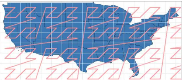
The TIGER shapefiles contain vector geospatial data. Both shapefiles (.shp) and database files (.dbf) are separated into census blocks by a hierarchical framework that groups files depending on their spatial coverage, such as nation, state and county-based files. The shapefiles include polygon boundaries of geographic areas, linear features (roads, hydrography and others) and point features. They do not contain any sensitive data, areas used for administering censuses, military information, surveys and other internal processing attributes. Figure 4.1 shows a portion of the vector dataset in the QGIS4 map viewer. The dataset classes are presented in Table 4.2.
4
4.2. Dataset 33 Table 4.2: 2013 TIGER/Line vector collections.
Folder Name Shapefile/Relationship File
ADDR Address Range Relationship File ADDRFEAT Address Range Feature
ADDRFN Address Range-Feature Name Relationship File
AIANNH American Indian/Alaska Native/Native Hawaiian Areas AITSN American Indian Tribal Subdivision National
ANRC Alaska Native Regional Corporation AREALM Area Landmark
AREAWATER Area Hydrography
BG Block Group
CBSA Metropolitan Statistical Area / Micropolitan Statistical Area CD Congressional District
CNECTA Combined New England City and Town Area COASTLINE Coastline
CONCITY Consolidated City
COUNTY County
COUSUB County Subdivision CSA Combined Statistical Area
EDGES All Lines
ELSD Elementary School District
ESTATE Estates
FACES Topological Faces (Polygons With All Geocodes) FACESAH Topological Faces-Area Hydrography Relationship File FACESAL Topological Faces-Area Landmark Relationship File FACESMIL Topological Faces-Military Installation Relationship File FEATNAMES Feature Names Relationship File
LINEARWATER Linear Hydrography METDIV Metropolitan Division MIL Military Installation
NECTA New England City and Town Area
NECTADIV New England City and Town Area Division OTHERID Other Identifiers
PLACE Place
POINTLM Point Landmark PRIMARYROADS Primary Roads
PRISECROADS Primary and Secondary Roads PUMA Public Use Microdata Area
RAILS Rails
ROADS All Roads
SCSD Secondary School District
SLDL State Legislative District –Lower Chamber SLDU State Legislative District –Upper Chamber STATE State and Equivalent
SUBBARRIO SubMinor Civil Division (Subbarrios in Puerto Rico) TABBLOCK Tabulation (Census) Block
TBG Tribal Block Group TRACT Census Tract TTRACT Tribal Census Tract UAC Urban Area/Urban Cluster UNSD Unified School District
34 Chapter 4. Comparison Methodology
4.3
Data Modeling
Many spatial data modeling methods extend the entity-relationship model for describ-ing geographic data. While the result of such data model extensions is usually as-sociated with relational database management systems, other non-relational spatial solutions are being used by very large GIS. With the NoSQL arrays taking over Big Data, data models that easily fit relational DBMS are being translated and adapted into other systems. However, this may not prove optimal when handling large amounts of data, as it is not so clear how to define which mapping strategy (or even more than one) to maintain, either on relational or non-relational DBMS. Modeling strategies based on the system requirements and features are necessary. Nonetheless, it is also important to evaluate how beneficial the adoption of multiple data mappings of the same dataset can be.
When modeling spatial attributes, one must consider that the association of primary and foreign keys applied to numbers and strings provides an easy way to join tables, which is not possible with geospatial attributes. Spatial data is a multi-dimensional attribute that by its nature is not a static join attribute, as the interaction between two spatial objects may generate more than two outcomes (some of which are not mutually exclusive) in opposition to the binary outcome of a numerical foreign key to the targeted numerical primary key. The outcome of such spatial relationships must be calculated dynamically as demonstrated next.
The model proposed by Clementini and Egenhofer [11, 17] became the standard procedure to associate two geospatial objects. It translates the relationship between two geometries into a set of outcomes based on a decision tree. An example of the outcome matrix, called the Dimensionally Extended nine-Intersection Model (DE-9IM) can be seen in Figure 4.2. Note that the intersection of the interiors is a two-dimensional area, so that matrix cell’s value equals 2, indicating that the object resulting from that operation is a two-dimension object, in other words, a polygon. When intersections are over single lines, that matrix cell’s value equals 1, indicating that a one dimensional object is the result. When the polygons touch over single points, that portion of the matrix equals 0, which indicates the 0-dimensional point objects as results. When there is no intersection between components, the respective matrix value is set to a Boolean false.
5
4.3. Data Modeling 35
Figure 4.2: DE-9IM over spatial object interactions5.
4.3.1
OMT-G
Considering that the spatial relations cannot be represented as foreign key associa-tions, Borges et al. [6] demonstrated how spatial data characteristics make modeling more complex and proposed the Object Modeling Technique for Geographic Applica-tions (OMT-G). The OMT-G provides conceptual, presentation and implementation abstraction levels and it is suitable for modeling spatial and non-spatial data in an organized way compatible with the Unified Modeling Language (UML6).
Figure 4.3 shows the OMT-G diagram representing the 2013/TIGER Line dataset main classes, including the generated collections for the urban network query set (Sub-section 4.3.3). The TIGER shapefile collection duplicates data in order to provide isolation between classes. This enables for the general public to download only the collections they require, as for example, being able to download the PRIMARYROADS subset without having to obtain the entire EDGES collection. This duplication of data also increases performance, as for example, when the most used EDGES subcategories are already in a separate table. Such design characteristic excludes the need for a table filter based on the EDGE attributes in order to verify if that EDGE object is a PRIMARYROAD or a LINEARWATER.
6
36 Chapter 4. Comparison Methodology
Figure 4.3: TIGER Line OMT-G main classes diagram.
4.3.2
Mapping Spatial Objects
When mapping spatial objects into DBMS, the relational systems usually end up with normalized tables (with some exceptions focusing on either performance or redundancy of data) and spatial columns, which is pretty much straightforward, as demonstrated in PostGIS. The attributes of spatial objects are translated into columns, and the spatial feature itself is a geometry type column. Objects of the same class are stored in their respective tables and the relationship between spatial objects is calculated dynamically through spatial functions and operators. The same does not apply to NoSQL DBMS, for which there might be more than one way to store multiple sets of data with relationships between them.
Considering the example of scientific papers and authors: In a relational DBMS, a usual mapping simply allocates one table regarding papers, another one authors
4.3. Data Modeling 37 paper contains its respective authors. It is important to notice that in both structures, there may be data duplication as the same paper may appear in more than one author document, as well as an author may be inserted in multiple paper objects.
Such problems led us to a common design implementation that focuses on avoid-ing document embeddavoid-ing, as it makes data alteration rather slow and might increase document size and data duplication. Specifically, the implementation allocates both
authorsandpapersinto two separate collections, with no document embedding. This example applies to the spatial attributes as well, in a way that it requires to dynamically calculate the relationship between two geospatial attributes.
Now focusing on the graph-oriented DBMS, every data item must be translated into either node or relationship attributes. Hence, every spatial object is added as a node to the graph. Nodes are then included in the spatial index through graph relationships. One exception regards the urban routing scenario, where spatial objects belonging to the EDGES collection became relationships as we will explain next.
4.3.3
Graph Mapping for Urban Routing
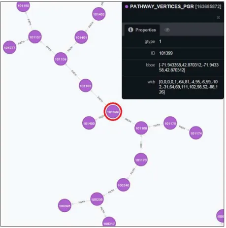
As detailed in Section 4.6, only PostgreSQL with pgRouting and Neo4j provide graph and network features. With that in mind, we have generated a fully traversable graph representing the United State’s automotive network. Specifically, objects that are in the EDGES table were filtered to produce the PATHWAY table. This data collection represents the same spatial attributes as the table ROADS, but the latter is not a fully traversable graph as it does not have road segments, rather full road linestrings. After filtering those objects from the EDGES table, we perform the pgRouting function for creating nodes based on those road segments. Those nodes translate into road inter-sections represented by the data collection PATHWAY_VERTICES_PGR. With both collections processed and indexed, we are able to perform graph operations, considering target, source and length of each EDGE (road segment).
38 Chapter 4. Comparison Methodology
4.4
Data Loading
During data loading, the dataset is read, processed and stored in disk. As mentioned earlier, we use the TIGER/Line vector dataset, which provides a large workload similar to many real world spatial databases, with enough data volume to represent a good spatial big data sample. The dataset contains more than 400 million objects, which requires efficient data loading. DBMS restoration and backup are a crucial part of any application’s database. Object coordinates in the dataset are originally encoded using the North American Datum of 1983 (NAD83), which we converted to the coordinates in the World Geodetic System 1984 (WGS84), the data used by the Global Positioning System (GPS). The conversion to both WGS84 and GeoJSON (used by MongoDB) was performed using the Geospatial Data Abstraction Library7.
All three DBMSs provide their own import tool (shp2pgsql in PostgreSQL, mon-goimport in MongoDB and Neo4j’sShapeFileImporter). Shp2pgsql performed very well right out of the box, translating shapefiles into PostgreSQL data relatively fast and without issues. However, the import tools provided by MongoDB and Neo4j were much slower, thus new tools were implemented to achieve a more reasonable import time. Also, as the import procedure is not executed as frequently as regular querying, data modification and backup routines, it is not part of the final performance evaluation. Detailed information about the improved data loading tools are described in Section 4.5.
After completing the dataset import, spatial indexes are created for all geometry fields. Indexes are also created for all attributes used in queries, such as road type (rural and local roads, highways and interstates) for urban routing, and point types for nearby points of interest. For MongoDB and Neo4j, our import tools generated the exact same database, with the same number of objects, with varying disk usage. For Neo4j, we were unable to compare the default import tool results, as its data importer was too slow: we canceled it after 72 hours of processing.
The disk space used by each DBMS compared to original files (shapefile and geojson) points out interesting behaviors. First by looking at data usage, it is clear that storing data as tables is much less expensive than documents and graphs. This happens because both graph and document systems store the key-value pair for each attribute, which is not necessary on relational systems as the key (column name) is not replicated on every object. Now regarding the disk space consumed by indexes, the generalized search tree (GiST) used by PostgreSQL is not as efficient as Neo4j’s graph strategy. MongoDB’s index disk consumption reflects the Geohash associated with a
7