Applying Piotroski’s F_Score to the German stock market: evidence from 2002-2016

(1)

FUNDAÇÃO GETÚLIO VARGAS

ESCOLA DE ECONOMIA DE EMPRESAS DE SÃO PAULO

PHILIPP MICHAEL DAMBACH

APPLYING PIOTROSKI’S F_SCORE TO THE GERMAN STOCK MARKET.

EVIDENCE FROM 2002-2016.

(2)

FUNDAÇÃO GETÚLIO VARGAS

ESCOLA DE ECONOMIA DE EMPRESAS DE SÃO PAULO

PHILIPP MICHAEL DAMBACH

APPLYING PIOTROSKI’S F_SCORE TO THE GERMAN STOCK MARKET.

EVIDENCE FROM 2002-2016.

SÃO PAULO

2016

Dissertação apresentada à Escola de

Economia de Empresas de São Paulo da

Fundação Getúlio Vargas, como requisito

para obtenção do título de Mestre

Profissional em Economia.

Campo do Conhecimento:

International Master in Finance

(3)

Dambach, Philipp Michael.

Applying Piotroski’s F_S

core to the German stock market: evidence from

2002-2016 / Philipp Michael Dambach. - 2002-2016.

47 f.

Orientadores: Ricardo Ratner Rochman, Pedro Lameira

Dissertação (MPFE) - Escola de Economia de São Paulo.

1. Mercado de capitais - Alemanha. 2. Ações (Finanças). 3. Investimento em valor.

4. Empresas - Avaliação. I. Rochman, Ricardo Ratner. II. Lameira, Pedro. III.

Dissertação (MPFE) - Escola de Economia de São Paulo. IV. Título.

(4)

PHILIPP MICHAEL DAMBACH

APPLYING PIOTROSKI’S F_SCORE TO THE GERMAN STOCK MARKET.

EVIDENCE FROM 2002-2016.

Dissertação apresentada à Escola de

Economia de Empresas de São Paulo da

Fundação Getúlio Vargas, como requisito

para obtenção do título de Mestre

Profissional em Economia.

Campo do Conhecimento:

International Master in Finance

Data de Aprovação:

_/_/____.

Banca Examinadora:

_________________________________

Prof. Dr. Ricardo R. Rochman

FGV-EESP

_________________________________

Prof. Dr. Pedro Lameira

NOVA SBE

_________________________________

Prof. Dr. Maria João Major

(5)

ACKNOWLEDGEMENTS

(6)

ABSTRACT

This work project applies Joseph Piotroski’s F_SCORE to the German stock market

between 2002 and 2016. Considering the smaller size of the German stock market, a

F_SCORE_ADD was created to differentiate between companies with the same score.

Portfolios that went long in expected winners and shorted expected losers generated

strong results within the small cap sample. For large caps, the abnormality of returns

was not significant after controlling for common risk factors and quality. This relates to

the results of other researchers and questions the practicality of the investment strategy

for institutional investors with a large capital base to employ.

(7)

RESUMO

Esta dissertação aplica o F_SCORE de Joseph Piotroski ao mercado de ações alemão

entre 2002 e 2016. Por causa do tamanho menor do mercado de ações alemão, um

F_SCORE_ADD foi criado para diferenciar entre as empresas com a mesma pontuação.

Carteiras que foram "long" em vencedores esperados e "short" em perdedores esperados

renderam bons resultados dentro da amostra com empresas de baixo valor de mercado.

Para as empresas de alta capitalização, a anormalidade de retornos não foi

estatisticamente significante após o controle de fatores de risco comuns e qualidade. Isto

relaciona-se com os resultados de outros investigadores e questiona a praticidade desta

estratégia de investimento para os investidores institucionais com uma grande base de

capital para empregar.

(8)

1. Introduction

p. 9

2. Literature Review

p. 11

3. Data and Methodology

p. 19

4. Results

p. 28

5. Summary and Conclusion

p. 38

6. Bibliography

p. 39

(9)

9

1. INTRODUCTION

(10)

10

order to gain further insights, quantitative strategies practice common diversification

principles. Different strategies were presented by practitioners and academic research

and tested for different markets.

(11)

11

2. LITERATURE REVIEW

Piotroski’s strategy relies upon a value and a quality component. The subsequent

literature review will present the academic foundation for these strategy determinants

before presenting Piotroski’s paper and the research related to it.

Systematic investing strategies try to profit from common market anomalies, of which

one of the most prominent is the value anomaly. The first authors to postulate an

investment strategy on a value basis are Graham/Dodd (1934). Since the publication of

their book “Security Analysis”, value investing evolved in many ways and nowadays

subsumes a whole pool of different strategies and approaches.

(12)

12

demonstrate that low price-to-book firms have higher average returns in the future.

Fama/French (1993) summarized that, different from prior academic theory, the average

returns on stocks cannot only be explained by the market factor by Sharpe (1964) but

also by size and book-to-market ratio which they considered in their three-factor model

for asset pricing.

Many explanations for the persistence of the value anomaly were suggested in the

literature. As a possible explanation De Bondt/Thaler (1985) presented in The Journal

of Finance that market overreaction leads to exceptionally large future returns of former

underperformers in terms of price-earnings ratios. They viewed this also as a proof for

substantial inefficiencies in the market. Research for the Japanese stock market by

Chan/Hamao/Lakonishkok (1991) proved that fundamental variables such as size, cash

flow, book-to-market ratio and price-to-book ratio have a significant impact on a firm’s

future earnings.

(13)

13

The other position is taken by Chen/Zhang (1998) who argued that value stocks are

riskier as they tend to be under distress, highly leveraged and have high uncertainty

concerning future earnings. The higher returns could be explained by these risk

attributes. The authors moreover found evidence that value stocks had higher returns in

many markets, but in high growth markets the spread tended to be smaller.

The second pillar for Piotroski’s strategy is the quality componen

t. The important

theoretical discussion is hereby, whether fundamentals can provide meaningful insights

about future stock returns and quality measurements can enhance the performance of the

value anomaly.

Ou/Penman (1989) delivered evidence that financial statements contain valuable

information about future earnings. They showed that with a contingent of financial

ratios from historic financial statement data, future changes in earnings can be

predicted. Engagement in stocks with a positive expected earnings change resulted in

abnormal returns that cannot be explained by firm risk characteristics or size.

Holthausen/Larcker (1992) also created a model based on fundamentals with which they

managed to predict future excess returns.

Research mentioned in the value anomaly section stated that high book-to-market stocks

tend to be neglected by analysts. Using fundamental analysis could therefore be

especially profitable in an environment with a low analyst-following as Piotroski (2000)

suggested.

(14)

14

strategy for the Shanghai Stock Exchange was delivered by Yangxiu (2013). However,

Wesley Gray and Tobias Carlisle (2013) argued that only the earnings yield is an

important factor and the inclusion of the return on capital factor actually lowers the

returns. This relates to similar arguments by Hsu and Kalesnik (2013) who concluded in

their research that quality measurements like gross profitability, return on equity or

gross margins are not robust and do not evidently carry a premium, whereas typical

value measurements like book-to-price, earnings-to-price or cashflow-to-price

persistently do.

On the other hand Asness et al. (2015) argued that controlling for quality helps for

example increasing the significance and performance of the size effect. Earlier,

Asness/Frazzini/Pedersen (2013) demonstrated that a quality factor that enables to

discriminate between “quality” and “junk” companies yields a positive premium and

can enhance the performance of value strategies. This revives the findings of

Lev/Thiagarajan (1993) and Abarbanell/Bushee (1998) who built an investment strategy

based on multiple fundamental signals that generated significant abnormal returns.

Fama/French (2014) updated their earlier three-factor model with two new variables;

they are considering profitability and investment patterns of companies as important

new factors for asset pricing.

(15)

15

Following up the mentioned research, Joseph Piotroski published his paper "Value

Investing: The Use of Historical Financial Statements to Separate Winners from Losers"

in 2000, introducing his fundamentally based quantitative strategy. Piotroski states that

even though low price-to-book stocks outperform on average, this is due only to a few

extremely well performing stocks while about 57% of these stocks in the sample

actually underperformed. He therefore introduces a F_SCORE, a signaling score based

on historical financial statement data that is meant to exclude those underperforming

stocks in order to shift the returns distribution of the portfolio rightwards. Piotroski

based himself on earlier research when selecting his screening variables. For example

Sloan (1996) suggested that investors tend to focus on earnings while neglecting the

information found in accruals and cash flow. This was incorporated in the ACCRUAL

variable. Loughran/Ritter (1995) found that companies that issue new shares

underperformed such ones that did not rely on this type of funding. This lead to the

EQ_OFFER variable. All determinants of the signals will be discussed further in the

methodology section. The fact that historical financial information can be used to

distinguish future winners and future losers is seen by Piotroski as a proof for stocks

prices not fully containing all historic signals.

(16)

16

strong and weak firms. The answer was yes, but the F_SCORE offered further

explanatory power. Other authors mentioned in the previous section provided similar

approaches based on aggregate fundamental data. This examination will follow the

original definitions of the F_SCORE in the further procedure.

Krüger/Beerstecher (2015) revisited Piotroski's F_SCORE strategy for the U.S market

for the recent period of time. They confirmed the high abnormal returns and proved that

those can only partially be explained by common risk factors. Nevertheless, they

considered the strategy to be unprofitable from a practical point of view as liquidity

constraints and trading costs inhibit investors from exploiting this anomaly. For

individual investors with limited capital the strategy might be sufficient but for

institutional investors it is not possible when one considers the amount of money they

have to invest.

Kim/Lee (2014) stressed that the results of Piotroski are likely to be overstated because

the accounting information of all firms would not be actually available for the given

point of time used in the study.

For the Mexican stock market, Dosamantes (2013) researched whether fundamental

strategies lead to positive excess market returns. He used signals based on accounting

fundamentals and then built portfolios with stocks that yield high scores. The research

specifically tested F_SCORE and the similar L_SCORE by Lev/Thiagarajan (1993).

The market excess annual returns were positive and significant even after controlling for

the FF3M factors, however, tended to decrease in the recent period of time.

(17)

17

performance for the subsequent years. They confirmed Piotroski's results for the

original sample period but stated that the following 12 years after the publication of the

paper showed reverse results, meaning that firms with a low F_SCORE outperformed

high F_SCORE stocks in the value stock segment and that stocks with a high F_SCORE

effectively underperformed the value segment as a whole. The robustness of these

results is still given after controlling for the size effect.

For the European stock market Amor-Tapia/Tascón (2016) tested different

fundamentally based composite indicators, namely F_SCORE2, PEIS, F_SCORE and

G_SCORE. Their findings are that only F_SCORE and G_SCORE, which is a

fundamental score developed for growth stocks, deliver abnormal returns. Most of the

returns are contributed by the short leg. However, they find evidence for limits of these

strategies in idiosyncratic risk, transaction costs and noise trader momentum risk.

Hyde (2014) analyzed the deployment of the F_SCORE strategy in emerging markets.

He demonstrated that high F_SCORE stocks indeed seem to offer a premium which

cannot be explained by value, size or momentum. He argues that the common

explanation that stocks with such a premium are neglected by analysts does not hold, as

high F_SCORE stocks are usually heavily followed and analyzed.

Singh and Kaur (2015) tested the Piotroski F_SCORE in the Indian stock market. Their

findings are that high F_SCORE stocks performed better than the sample of all value

stocks and delivered abnormal returns even after controlling for size, momentum, value,

recent equity offerings and accrual effects.

(18)

18

the efficacy using fundamental signals. Evidence about practicality and persistence

shows, however, mixed results. This work project tries to add to the discussion by

testing and developing the approach for the German stock market for the recent period

of time whilst trying to create an additional sorting signal that makes the method

applicable for smaller stock markets.

(19)

19

3. DATA AND METHODOLOGY

This work tries to contribute to the discussion of practicality of

Piotroski’s

investing

strategy by testing it on the German stock market. Therefore, the companies for the

sample are drawn from the CDAX index which contains all stock corporations in

Germany. The time horizon for the examination is 2002-2016, because reliable

information about the historical index constituents is only available from the beginning

of 2002 onwards. In addition, the focus is designed to lie on the recent years and

financial crises. The strategy requires portfolio updates every year. Therefore the first

step was to retrieve the Portfolio constituents at each year. This step is important in

order to ensure that the data is

as much “point in time” as possible. Using the current

constitution of the index would lead to a survivorship bias, because it excludes all

companies that got bankrupt or acquired throughout time.

Graph 1. Change in CDAX Index Constitution 2002-2015.

Graph 1 illustrates the extent to which the index constitution changed. In 2002 there

were 789 companies included in the CDAX index, whereas in 2015 only 446 companies

constitute the index. On average, the number of stocks in the index declined by 4.29%

789

737

709

681

675

690

682

653

618

583

554

511

484

446

400

450

500

550

600

650

700

750

800

850

(20)

20

annually. This proves the importance of using the actual index constitution of each

respective year.

The next step was to retrieve the financial statement data needed to build portfolios

based on Joseph Piotroski’s method.

All of the subsequent data was taken from

Bloomberg, unless marked differently. First, the companies were ranked each year

based on their price-to-book ratios. The F_SCORE was then calculated for the quintile

with the lowest price-to-book ratios. It represents an aggregate score that assesses

companies based on three key areas, namely profitability, financial performance and

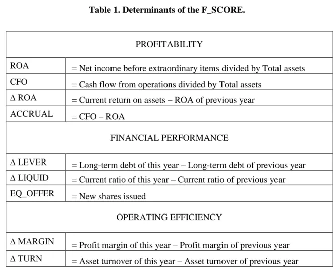
operating efficiency. Table 1 specifies the determinants of the F_SCORE within the

three key areas.

Table 1. Determinants of the F_SCORE.

PROFITABILITY

ROA

_{= Net income before extraordinary items divided by Total assets}

CFO

_{= Cash flow from operations divided by Total assets}

∆ ROA

_{= Current return on assets}

_–

_{ROA of previous year}

ACCRUAL

_{= CFO}

_–

_ROA

FINANCIAL PERFORMANCE

∆ LEVER

_{= Long-term debt of this year – Long-term debt of previous year}

∆ LIQUID

_{= Current ratio of this year – Current ratio of previous year}

EQ_OFFER

_{= New shares issued}

OPERATING EFFICIENCY

(21)

21

The first area in which the companies are assessed is the area of profitability. Positive

ROA and CFO can be seen as a positive sign when considering the poor earnings

history of most value firms. Also any improvement in ROA is considered as a positive

signal. The ACCRUAL variable reflects positive accrual adjustments, which Sloan

(1996) showed to have a significant negative impact on future returns. Piotroski defines

it as profits being greater than cash flow from operations. Whenever the opposite is the

case it should be seen as a positive signal.

The next area is financial performance, which focuses on assessing changes in the

capital structure. The first variable subsumes the change in long-term debt levels.

Piotroski states that when distressed firms raise capital externally, this should be seen as

a proof that they cannot generate enough funding internally. Moreover it makes the

firms less financially flexible. The positive change in current ratio adresses the liquidity

and should be seen as a positive signal when it is achieved. Following Loughran/Ritter

(1995), who found that new-share-issuers tend to underperform, results in a disapproval

for new shares in the EQ_OFFER variable. This also addresses the earlier point of

external financing representing a lack of internal financing possibilities.

The last section deals with the operating efficiency of the respective companies.

The

two variables used are changes in gross margin and asset turnover. An improved gross

margin ratio indicates cost reduction or a higher price for the products sold. A higher

asset turnover is a sign for productivity improvements such as higher sales or an

increase in the efficiency of a firm’s operations.

(22)

22

instance, additional leverage would not necessarily result in a negative signal. Table 2

explains all of the nine resulting binary signals that follow these determinants.

Table 2. Binary Signals from the Determinants of the F_SCORE.

𝑰

𝑨 > ,

𝑨

= { ,

𝑰

> ,

= { ,

𝑰 ∆

𝑨 > ,

∆𝐑 𝑨

= { ,

𝑰 𝑨

𝑨 > ,

𝑨

= { ,

𝑰 ∆ 𝐕 𝐑 < ,

∆ 𝐕 𝐑

= { ,

𝑰 ∆ 𝐈𝐐𝐔𝐈 > ,

𝑨

= { ,

𝑰

≤ ,

_

= { ,

𝑰 ∆ 𝐀𝐑𝐆𝐈 > ,

∆ 𝐀𝐑𝐆𝐈

= { ,

(23)

23

With the F_SCORE being the sum of the individual binary signals it can be described

with the following equation. The highest possible score is accordingly 9 for a company

with very strong prospects and 0 for a company of extremely low quality.

Equation 1. Composition of the F_SCORE.

_

=

𝑨

+

∆

𝑨

+

𝑨

+

∆

+

∆ 𝑰

𝑰

+

∆ 𝑨

𝑰

+

∆

Piotroski acknowledges that using simple binary signals could lead to an elimination of

useful information. Furthermore, in some years many companies may have the same

score, whereas other scores are relatively underrepresented. Because the German stock

index is considerably smaller than the U.S. company horizon, this imposes restrictions

on the original way Piotroski formed his portfolios. Instead of bundling companies with

the same score into portfolios, this paper will work with deciles and quintiles. The

reason is to ensure enough diversification as high and low F_SCORE ranks tend to be

rarer than mediocre F_SCOREs.

(24)

24

Table 3. Strength Determinants for F_SCORE_ADD.

𝑰

𝑨 > , 𝑨

𝑨

= {

𝑨,

𝑰

> , 𝑨

= {

,

𝑰 ∆

𝑨 > , 𝑨

∆𝐑 𝑨

= {∆

𝑨,

𝑰 𝑨

𝑨 > , 𝑨

𝑨

= {

−

𝑨,

𝑰 ∆ 𝐕 𝐑 < , 𝑨

∆ 𝐕 𝐑

= {−∆ 𝐕 𝐑,

𝑰 ∆ 𝐈𝐐𝐔𝐈 > , 𝑨

𝑨

= {∆ 𝐈𝐐𝐔𝐈 ,

𝑰

≤ , 𝑨

= { ,

𝑰 ∆ 𝐀𝐑𝐆𝐈 > , 𝑨

∆ 𝐀𝐑𝐆𝐈

= {∆ 𝐀𝐑𝐆𝐈 ,

𝑰 ∆

> , 𝑨

∆𝐓𝐔𝐑

= {∆

,

Whenever a condition is fulfilled that would lead to a positive F_SCORE signal, the

amount of positiveness is considered, for example how much the return on assets

improved compared to the previous year.

(25)

25

Equation 2. Composition of the F_SCORE_ADD.

_

_𝑨

= (

_{𝒂𝒍 𝑨}

) ∗ 𝑨

𝑨

+ 𝑨

∆

𝑨

+ 𝑨

𝑨

+ 𝑨

∆

+ 𝑨

∆ 𝑰

𝑰

+ 𝑨

∆ 𝑨

𝑰

+ 𝑨

∆

After ranking all companies in the low price-to-book ratio quintile based on first

F_SCORE and then F_SCORE_ADD, portfolios were created based on deciles and

quintiles. For instance, the highest ranked decile in each year would stand for a

portfolio. Within each portfolio, all assets are assumed to be equally weighted.

In order to examine, whether the results are different for large and small corporations,

the sample was also split between companies of less

than 100 million € market

capitalization and such that have a higher market capitalization. The same procedure

mentioned above was then performed analogously for these two sample splits.

After determining the portfolios, the logged total return of each portfolio, which is

defined in equation 3, was calculated on a monthly basis.

Equation 3. Calculation of Returns.

= 𝒍 (

+

−

)

(26)

26

calculated using the price to which they got delisted, the return of acquired companies

was calculated using the price for which they got acquired.

After calculating the decile returns, the CAPM, Fama-French three- and five-factor

models (FF3M and FF5M), the Carhart four-factor model (C4FM), the FF3M plus the

QMJ factor (Q4FM) and the C4FM plus the QMJ factor, which will be defined as

Q5FM further in the text, were used in order to see if the strategy generates significant

alpha after controlling for common risk factors and quality. The models were defined as

follows, with rit

resembling the excess portfolio return after adjusting for the risk-free

rate, which is proxied by the average one month money market rates (“Monatsgeld”) for

the beginning of the sample period and the one-month EURIBOR after June 2012.

CDAXRF is the excess return on the CDAX; SMB, HML, WML, RMW, CMA and

QMJ are returns on zero-investment, factor-mimicking portfolios for size,

book-to-market, momentum, profitability, investment patterns and quality.

CAPM:

𝑟

_𝑖𝑡

=

α

_𝑖𝑇

+ 𝑏

_𝑖𝑇

𝐶𝐷𝐴𝑋𝑅𝐹

_𝑡

+ 𝑒

_𝑖𝑡

FF3M:

𝑟

_𝑖𝑡

=

α

_𝑖𝑇

+ 𝑏

_𝑖𝑇

𝐶𝐷𝐴𝑋𝑅𝐹

_𝑡

+ 𝑠

_𝑖𝑇

𝑆𝑀𝐵

_𝑡

+ ℎ

_𝑖𝑇

𝐻𝑀𝐿

_𝑡

+ 𝑒

_𝑖𝑡

C4FM:

𝑟

_𝑖𝑡

=

α

_𝑖𝑇

+ 𝑏

_𝑖𝑇

𝐶𝐷𝐴𝑋𝑅𝐹

_𝑡

+ 𝑠

_𝑖𝑇

𝑆𝑀𝐵

_𝑡

+ ℎ

_𝑖𝑇

𝐻𝑀𝐿

_𝑡

+ 𝑤

_𝑖𝑇

𝑊𝑀𝐿

_𝑡

+ 𝑒

_𝑖𝑡

Q4FM:

𝑟

_𝑖𝑡

=

α

_𝑖𝑇

+ 𝑏

_𝑖𝑇

𝐶𝐷𝐴𝑋𝑅𝐹

_𝑡

+ 𝑠

_𝑖𝑇

𝑆𝑀𝐵

_𝑡

+ ℎ

_𝑖𝑇

𝐻𝑀𝐿

_𝑡

+ 𝑞

_𝑖𝑇

𝑄𝑀𝐽

_𝑡

+ 𝑒

_𝑖𝑡

Q5FM:

𝑟

_𝑖𝑡

=

α

_𝑖𝑇

+ 𝑏

_𝑖𝑇

𝐶𝐷𝐴𝑋𝑅𝐹

_𝑡

+ 𝑠

_𝑖𝑇

𝑆𝑀𝐵

_𝑡

+ ℎ

_𝑖𝑇

𝐻𝑀𝐿

_𝑡

+ 𝑤

_𝑖𝑇

𝑊𝑀𝐿

_𝑡

+ 𝑞

_𝑖𝑇

𝑄𝑀𝐽

_𝑡

+ 𝑒

_𝑖𝑡

FF5M:

𝑟

_𝑖𝑡

=

α

_𝑖𝑇

+ 𝑏

_𝑖𝑇

𝐶𝐷𝐴𝑋𝑅𝐹

_𝑡

+ 𝑠

_𝑖𝑇

𝑆𝑀𝐵

_𝑡

+ ℎ

_𝑖𝑇

𝐻𝑀𝐿

_𝑡

+ 𝑟

_𝑖𝑇

𝑅𝑀𝑊

_𝑡

+ 𝑐

_𝑖𝑇

𝐶𝑀𝐴

_𝑡

+ 𝑒

_𝑖𝑡

(27)

27

of this multi-factor data set is delivered by Brückner et al. (2015).

1

Because the German

factor data set only reaches until June 2015, the missing year

’s

factors are proxied with

the Fama/French European data set provided by Kenneth French.

2

_{This also applies for}

the two additional factors used for the Fama-French five-factor Model. The German

QMJ factors were retrieved from the data set provided by AQR which is related to the

paper by Asness/Frazzini/Pedersen (2013).

3

1 _Source:

https://www.wiwi.hu-berlin.de/de/professuren/bwl/bb/data/fama-french-factors-germany/fama-french-factors-for-germany

(28)

28

4. RESULTS

The following section will present the results of the examination. First, tables with the

raw returns will show the performance of each decile and quintile of the sample, both

for the whole sample size as well as for large caps and small caps respectively.

Thereafter, the results of benchmarking the excess returns over the risk free rate of the

three samples with common risk factors and quality will be summarized and discussed.

Table 3. Descriptive Statistics of Returns

–

Whole Sample Size.

(29)

29

(30)

30

The next paragraphs will discuss the difference of performance in large and small caps.

For this examination the sample was split in half between companies that exceed a

market capitalization of 100 million € and such that do not.

Splitting the sample leads to

a smaller sample base, because Piotroski’s method works with the bottom quintile of

price-to-book companies. Therefore the resulting portfolios contain less companies,

which impacts diversification effects. This should be kept in mind when comparing the

following results to the results for the whole sample size.

Table 4. Descriptive Statistics of Returns

–

Large Caps.

(31)

31

However, the relationship between number of decile and returns are less perfect, even

when looking at quintiles. This is mainly due to the fact that the 7

th

decile is the best

performing one, which proves that the Piotroski F_SCORE has a more limited

application among large corporations with a probably high analyst following. As a

result, the long-short portfolios have lower information Sharpe ratios compared to the

whole sample size portfolios, the average being 0.75. Distribution of returns and higher

moments do not show the same characteristics as in the whole sample size. More

portfolios exhibit negative skewness and for some the monthly maximum does not

outstrip the monthly minimum. Also, the percentage of positive years is lower.

(32)

32

Table 5 summarizes the statistics for the small cap sample. Of all three samples, it offers

the highest return for the top decile and quintile. The relationship between F_SCORE

and F_SCORE_ADD rank and returns is more stringent than for the large cap sample.

In the quintiles however, the relationship appears not perfect due to the large negative

performance of the 8

th

decile. The distribution of returns seems more extreme in the

small cap sample with some deciles having high monthly maxima and minima and

extreme kurtosis figures. Also, the numbers of positive years and months are the lowest

for this sample. The long-short porfolios offer higher information Sharpe ratios of

around one compared to the large cap sample. Also the spread between high F_SCORE

and low F_SCORE companies is the highest in this sample, resulting in an average

return of 32.39% for the portfolio that goes long in the top decile and short in the

bottom decile. The long-short portfolios exhibit monthly maxima that largely exceed the

monthly minima. Also, the skewness for all portfolios is positive and almost all

portfolios have a leptokurtic distribution. The number of positive months is high and the

portfolios offered positive results in almost all years of the period studied.

(33)

33

for this sample, especially when one considers the half-year lag between the end of a

financial year and the actual investment period. Small caps showed a more stringent

relationship between F_SCORE rank and performance. Therefore the risk-return metrics

are more attractive. On the other hand, the small cap sample exhibits more extreme

statistics, with high kurtosis figures and mostly negative deciles for the long only

portfolios. Also, the majority of returns is yielded by the short leg. It seems that these

companies are more distressed and in a worse state compared to the large cap

companies. Also, these companies appear less investible due to the fact that they are of

a low market capitalization. This may impose liquidity constraints and high transaction

costs, which may make investing in these companies with the Piotroski method

unfeasible. On the other hand, this may be also the reason for the profitability of

investing in this segment with the F_SCORE method, as fundamental data does not get

incorporated as fast.

The next step was to benchmark the returns with common factor models. Six different

regressions were performed. The first one is the Capital Asset Pricing Model by Sharpe

(1964), the second one is the Fama-French three-factor model by Fama/French (1996),

the third one their extended five-factor model (2014), the fourth one is the four-factor

model by Carhart (1997), the fifth one is the Q4FM, which resembles the FF3M

extended

with

a

quality-minus-junk

factor

(QMJ)

introduced

by

Asness/Frazzini/Pedersen (2013), and the sixth one is the Q5FM, which will resemble

the C4FM extended with the QMJ factor. Three summary tables for each sample will be

presented and discussed, the regression output can be found in the the appendix.

4

(34)

34

Table 6. Regression Summary for Long-Short Portfolios

–

Whole Sample Size.

5

Table 6 summarizes the regression outputs for the portfolios drawn from the complete

sample size. Controlling the excess returns of the five long-short portfolios over the

risk-free rate for the risk-adjusted market return, size, value, momentum, quality,

profitability and investment patterns results in a positive and significant alpha at the 5%

5 _{For all three regression summary tables the following symbols mark the significance of the variables.}

*

Significant at the 1% level

** Significant at the 5% level

***

Significant at the 10% level

X Not significant

Model:

Whole Sample Size

(1)–(10)

(1-2)–(9-10) (1-3)–(8-10) (1-4)–(7-10) (1-5)–(6-10)

CAPM:

α

*

CDAX-Rf

X

*

FF3M:

α

*

CDAX-Rf

X

*

**

SMB

X

HML

X

C4FM:

α

*

CDAX-Rf

X

***

X

SMB

X

HML

X

WML

X

***

**

Q4FM:

α

*

**

*

CDAX-Rf

X

SMB

X

HML

X

QMJ

X

***

X

Q5FM:

α

*

**

CDAX-Rf

X

SMB

X

HML

X

WML

X

***

QMJ

X

FF5M:

α

*

**

CDAX-Rf

X

SMB

X

HML

X

RMW

X

**

*

**

(35)

35

level for all portfolios in all models. Adding quality factors or controlling for the

profitability and the investment patterns of the companies does not manage to eliminate

the alpha achieved by Piotroski’s method.

Interestingly, the RMW factor by

Fama/French (2014) performed better as a variable than the QMJ factor by

Asness/Frazzini/Pedersen (2013).

Table 7. Regression Summary for Long-Short Portfolios

–

Large Caps.

Model:

Large Cap Sample

(1)–(10)

(1-2)–(9-10) (1-3)–(8-10) (1-4)–(7-10) (1-5)–(6-10)

CAPM:

α

*

**

CDAX-Rf

*

**

***

FF3M:

α

*

**

CDAX-Rf

*

***

SMB

**

*

**

X

HML

X

**

X

C4FM:

α

**

*

X

CDAX-Rf

**

*

**

X

SMB

**

X

HML

X

**

***

X

WML

X

*

**

Q4FM:

α

***

*

X

CDAX-Rf

X

**

X

SMB

**

*

X

HML

X

***

*

X

QMJ

***

*

***

X

Q5FM:

α

***

X

**

X

CDAX-Rf

X

SMB

***

X

HML

X

***

X

WML

X

*

**

***

QMJ

X

*

X

FF5M:

α

**

*

***

CDAX-Rf

*

***

X

SMB

**

***

X

HML

X

***

X

RMW

X

***

X

(36)

36

For the large cap sample controlling for common risk factors and quality diminishes the

alpha obtained by Piotroski’s F_SCORE

strategy. In contrast to the whole sample size,

the QMJ factor hereby explains the returns better than the RMW factor. A possible

explanation could be that the QMJ factor by Asness/Frazzini/Pedersen (2013) is derived

from the Gordon growth model, which may be more suitable for large corporations. The

Q5FM model seems to capture the returns the best.

Table 8. Regression Summary for Long-Short Portfolios

–

Small Caps.

Model:

Small Cap Sample

(1)–(10)

(1-2)–(9-10) (1-3)–(8-10) (1-4)–(7-10) (1-5)–(6-10)

CAPM:

α

*

CDAX-Rf

**

*

**

FF3M:

α

*

CDAX-Rf

**

*

SMB

X

HML

X

***

X

***

C4FM:

α

*

CDAX-Rf

**

*

**

SMB

X

HML

X

***

X

***

WML

X

Q4FM:

α

*

CDAX-Rf

**

X

***

X

SMB

X

HML

X

***

X

QMJ

X

Q5FM:

α

*

CDAX-Rf

**

X

***

X

SMB

X

HML

X

***

X

WML

X

QMJ

X

FF5M:

α

*

CDAX-Rf

**

***

X

SMB

X

HML

X

***

X

RMW

X

***

(37)

37

In the small cap sample the alpha for all portfolios is significant above the 1% level.

The only significant variable above the 10% level is the excess return of the CDAX

over the risk-free rate. Controlling for common risk factors, quality, profitability and

investment patterns does not affect the abnormality of returns in this sample.

All long-short portfolios show a small and negative beta towards the market excess

return. This means that the returns of these portfolios are not very and negatively

correlated with market movements, which could provide attractive characteristics, when

added to a portfolio that has considerable market risk. Splitting the sample revealed that

the long cap sample with corporations of a market capitalization above 100 million €

(38)

38

5. SUMMARY AND CONCLUSION

The systematic quantitative investment method based on Piotroski

’s

F_SCORE yielded

positive and stable results in the German stock market for the sample period of

2002-2016. Using a F_SCORE_ADD appeared a viable way to expand the application of the

Piotroski F_SCORE to smaller stock markets. Further research can contribute to the

discussion of this extension of the F_SCORE.

A portfolio that goes long in expected winners and shorts expected losers based on

fundamental signals for stocks within the highest book-to-market quintile of the CDAX

index generated high abnormal returns even after controlling for common risk factors

and quality. In fact, the portfolio returns had very little and negative correlation with the

market and the strategy appeared stable throughout the sample period.

(39)

39

6. BIBLIOGRAPHY

Abarbanell, Jeffrey, and Brian Bushee.

1997. “

Fundamental Analysis, Future

Earnings, and Stock Prices.”

Journal of Accounting Research, 35: 1-24.

Abarbanell, Jeffrey, and Brian Bushee.

1998. “

Abnormal Returns to a Fundamental

Analysis Strategy

”

. Accounting Review, 73: 19-45.

Altman, Edward. 1968. “Financial Ratios, Discriminant analysis and the Prediction of

Corporate Bankruptcy.” The Journal of Finance, 23(4): 589-609.

Amor-Tapia, Borja, and María Tascón.

2016. “

Separating Winners from Losers:

Composite Indicators Based on Fundamentals in the European Context.” Journal of

Economics and Finance, 66(1): 70-94.

Asness, Clifford, Andrea Frazzini, and Lasse Pedersen.

2013. “Quality Minus Junk

.

”

Working Paper.

Asness, Clifford, Andrea Frazzini, Ronen Israel, Tobias Moskowitz, and Lasse

Pedersen.

2015. “Size Matters, If You Control Your Junk.”

Working Paper.

Basu, Sanjoy. 1977. “Investment Performance of Common Stocks in Relation to their

Price-

Earnings Ratios: A Test of the Efficient Market Hypothesis.”

The Journal of

Finance, 32(3): 663-682.

Basu, Sanjoy. 1983. “The relationship between earnings' yield, market value and return

for NYSE common stocks: Further evidence.”

Journal of Financial Economics, 12(1):

129-156.

Brückner, Roman, Patrick Lehmann, Martin Schmidt, and Richard Stehle. 2015.

“

Another German Fama/French Factor Data Set

.”

http://ssrn.com/abstract=2682617.

Campbell, John, and Robert Shiller.

1988. “Stock Prices, Earnings, and Expected

Dividends.”

The Journal of Finance, 43(3): 661-676.

Carhart, Mark.

1997. “

On Persistence in Mutual Fund Performance.

”

The Journal of

Finance, 52(1): 57-82.

Chan, Louis, Yasushi Hamao, and Josef Lakonishok.

1991. “Fundamentals and

Stock Returns in Japan.”

The Journal of Finance 46(5): 1739-1789.

Chen, Nai-fu, and Feng Zhang. 1998. “Risk and Return of Value Stocks.”

Journal of

Business, 71(4): 501-535.

De Bondt, Werner, and Richard Thaler.

1985. “Does the Stock Market Overreact?”

The Journal of Finance, 40(3): 793-805.

(40)

40

Fama, Eugene, and Kenneth French.

1992. “The Cross-Section of Expected Stock

Returns.” The Journal of Finance, 47(2): 427-465.

Fama, Eugene, and Kenneth French.

1996. “

Multifactor Explanations of Asset

Pricing Anomalies.” The Journal of Finance, 51(1): 55-84.

French, Eugene, and Kenneth French.

2014. “

A Five-Factor Asset Pricing Model

.”

Fama-Miller Working Paper.

Fama, Eugene, and Marshall Blume. 1966. “Filter Rules and Stock-Market Trading.”

The Journal of Business, 39(1): 226-241.

Graham, Benjamin, and David Dodd. 1934. Security Analysis. New York:

McGraw-Hill.

Gray, Wesley, and Tobias Carlisle. 2013. Quantitative Value: A Practitioner's Guide

to Automating Intelligent Investment and Eliminating Behavioral Errors. Hoboken,

New Jersey: John Wiley & Sons.

Greenblatt, Joel. 2006. The Little Book That Beats the Market. Hoboken, New Jersey:

John Wiley & Sons.

Haugen, Robert, and Nardin Baker.

1996. “Commonality in the Determinants of

Expected Stock Returns.”

Journal of Financial Economics, 41: 401.

Holthausen, Robert, and David Larcker.

1996. “The Prediction of Stock Returns

Using Financial Statement Information.”

Journal of Accounting and Economics 15(3):

373-411.

Hsu, Jason, and Vitali Kalesnik. 2014. Finding Smart Beta in the Factor Zoo.

Newport Beach, California: Research Affiliates.

Hyde, Charles.

2014. “

An Emerging Markets Analysis of the Piotroski F-

score.”

The

Finsia Journal of Applied Finance, 2: 23-28.

Jaffe, Jeffrey, Donald Keim, and Randolph Westerfield.

1989. “Earnings Yields,

Market Valu

es, and Stock Returns.”

The Journal of Finance, 44(1): 135-148.

Kim, Sohyung, and Cheol Lee.

2014. “

Implementability of Trading Strategies Based

on Accounting Information: Piotroski (2000) Revisited.” European Accounting Review,

23(4): 553-558.

Kothari, Suthawan.

2001. “Capital

markets research in accounting.” Journal of

Accounting and Economics, 31(1-3): 105-231.

Krauss, Christopher, Tom Krüger, and Daniel Beerstecher.

2015. “

The Piotroski

F-Score: A fundamental value strategy revisited

from an investor's perspective.” IWQW

Discussion Paper Series, 13: 1-27.

La Porta, Rafael, Josef Lakonishok, Andrei Shleifer, and Robert Vishny. 1997.

“Good News for Value Stocks: Further Evidence on Market Efficiency.” The Journal of

(41)

41

Lev, Baruch, and S. Ramu Thiagarajan. 1993. “Fundamental Information Analysis.”

Journal of Accounting Research, 31(2): 190-215.

Loughran, Tim, Jay Ritter.

1995. “The New Issues Puzzle.”

The Journal of Finance,

50(1): 23-51.

Ou, Jane, and Stephen H. Penman. 1989

. “Accounting Measurement, Price

-Earnings

Ratio, and the Information Content of Security Prices.”

Journal of Accounting

Research, 27: 111-144.

Ou, Jane, and Stephen H. Penman. 1989

. “Financial Statement Analysis and the

Prediction of Stock Returns.”

Journal of Accounting and Economics, 11: 295-329.

Piotroski, Joseph. 2000. “Value Investing: The Use of Historical Financial Statements

to Separate Winners from Losers.” Journal of Accounting Research, 38.

Piotroski, Joseph, and Eric So.

2011. “

Identifying Expectation Errors in

Value/Glamour Strategies: A

Fundamental Analysis Approach.” Review of Financial

Studies, 25(9): 2841-2875.

Rosenberg, Barr, Kenneth Reid, and Ronald Lanstein. 198

5. “

Persuasive Evidence

of Market Inefficiency.” Journal of Portfolio Management, 11: 9-17.

Scatizzi, Cara.

2010. “

Adjusting for the real world: Testing variations of Piotroski's

Screen.

”

AAII Journal, 32(4): 21-26.

Sharpe, William. 1964. “Capital Asset Prices: A Theory of Market Equilibrium under

Conditions of Risk.”

The Journal of Finance, 19(3): 425-442.

Singh, Jaspal, and Kiranpreet Kaur.

2015. “Adding value to value stocks in Indian

stock

market: an empirical analysis.” International Journal of Law and Management,

57(6): 621-636.

Sloan, Richard.

1996. “Do Stock Prices Fully Reflect Information in Accruals and

Cash Flows about Future Earnings?”

The Accounting Review, 71(3): 289-315.

Stattman, Dennis.

1980. “Book Values and Stock Returns.”

The Chicago MBA: A

Journal of Selected Papers, 4: 25-45.

Stickel, Scott.

1998. “Analyst Incentives and the Financial Characteristics of Wall

Street Darlings and Dogs.”

The Journal of Investing, 16(3): 23-32.

Woodley, Melissa, Steven Jones, and James Reburn.

2011. “Value Stocks and

Accounting Screens: Has a Good Rule Gone Bad?” Journal of Accounting and Finance,

11(4): 87-104.

(42)

42

7. APPENDICES

8.

Table 9. Long-Short Portfolio Regressions

–

Output for Whole Sample Size.

Dependent Variable: _1___10_ Method: Least Squares Date: 08/01/16 Time: 20:13 Sample: 2002M07 2016M06 Included observations: 168

Variable Coefficient Std. Error t-Statistic Prob.

C 0.021675 0.005438 3.985769 0.0001

CDAX_RF -0.097067 0.089209 -1.088088 0.2781

R-squared 0.007082 Mean dependent var 0.021296

Adjusted R-squared 0.001100 S.D. dependent var 0.070379

S.E. of regression 0.070340 Akaike info criterion -2.459113

Sum squared resid 0.821326 Schwarz criterion -2.421923

Log likelihood 208.5655 Hannan-Quinn criter. -2.444019

F-statistic 1.183935 Durbin-Watson stat 2.133867

Prob(F-statistic) 0.278134

Dependent Variable: _1_2___9_10_ Method: Least Squares Date: 08/01/16 Time: 20:14 Sample: 2002M07 2016M06 Included observations: 168

C 0.017103 0.004028 4.245558 0.0000

CDAX_RF -0.226440 0.066085 -3.426505 0.0008

C 0.014078 0.003760 3.743827 0.0002

CDAX_RF -0.172723 0.061688 -2.799971 0.0057

C 0.011118 0.003004 3.701318 0.0003

CDAX_RF -0.148008 0.049276 -3.003631 0.0031

C 0.009770 0.002686 3.638085 0.0004

CDAX_RF -0.125699 0.044056 -2.853181 0.0049

Variable Coefficient Std. Error t-Statistic Prob. C 0.020777 0.005551 3.743193 0.0003 CDAX_RF -0.116353 0.098582 -1.180271 0.2396 SMB -0.072528 0.188271 -0.385233 0.7006 HML 0.160767 0.210653 0.763182 0.4465 R-squared 0.012351 Mean dependent var 0.021296 Adjusted R-squared -0.005715 S.D. dependent var 0.070379 S.E. of regression 0.070580 Akaike info criterion -2.440625 Sum squared resid 0.816967 Schwarz criterion -2.366245 Log likelihood 209.0125 Hannan-Quinn criter. -2.410438 F-statistic 0.683655 Durbin-Watson stat 2.121551 Prob(F-statistic) 0.563235

C 0.016968 0.004119 4.119211 0.0001

CDAX_RF -0.242847 0.073157 -3.319512 0.0011

SMB -0.073278 0.139715 -0.524481 0.6007

HML 0.005229 0.156325 0.033453 0.9734

C 0.013503 0.003833 3.522881 0.0006

CDAX_RF -0.199794 0.068074 -2.934939 0.0038

SMB -0.114415 0.130008 -0.880062 0.3801

HML 0.082357 0.145463 0.566168 0.5721

C 0.010956 0.003070 3.568395 0.0005

CDAX_RF -0.162087 0.054530 -2.972422 0.0034

SMB -0.062038 0.104141 -0.595714 0.5522

HML 0.014072 0.116522 0.120771 0.9040

C 0.009572 0.002746 3.485752 0.0006

CDAX_RF -0.119960 0.048773 -2.459582 0.0149

SMB 0.030149 0.093145 0.323681 0.7466

HML 0.049498 0.104219 0.474942 0.6355

Variable Coefficient Std. Error t-Statistic Prob. C 0.018745 0.005720 3.277243 0.0013 CDAX_RF -0.029499 0.116072 -0.254142 0.7997 SMB -0.009270 0.193022 -0.048025 0.9618 HML 0.168883 0.210106 0.803798 0.4227 WML 0.170998 0.121556 1.406747 0.1614 R-squared 0.024198 Mean dependent var 0.021296 Adjusted R-squared 0.000252 S.D. dependent var 0.070379 S.E. of regression 0.070370 Akaike info criterion -2.440787 Sum squared resid 0.807167 Schwarz criterion -2.347812 Log likelihood 210.0261 Hannan-Quinn criter. -2.403054 F-statistic 1.010536 Durbin-Watson stat 2.095851 Prob(F-statistic) 0.403682

Variable Coefficient Std. Error t-Statistic Prob. C 0.014936 0.004224 3.536374 0.0005 CDAX_RF -0.156027 0.085710 -1.820410 0.0705 SMB -0.010045 0.142531 -0.070478 0.9439 HML 0.013343 0.155147 0.086000 0.9316 WML 0.170930 0.089759 1.904312 0.0586 R-squared 0.088015 Mean dependent var 0.016220 Adjusted R-squared 0.065635 S.D. dependent var 0.053757 S.E. of regression 0.051963 Akaike info criterion -3.047273 Sum squared resid 0.440119 Schwarz criterion -2.954298 Log likelihood 260.9709 Hannan-Quinn criter. -3.009539 F-statistic 3.932764 Durbin-Watson stat 1.965896 Prob(F-statistic) 0.004481

C 0.011210 0.003909 2.867353 0.0047

CDAX_RF -0.101791 0.079335 -1.283043 0.2013

SMB -0.043036 0.131931 -0.326206 0.7447

HML 0.091515 0.143608 0.637257 0.5249

WML 0.192948 0.083083 2.322348 0.0215

C 0.009283 0.003140 2.955953 0.0036

CDAX_RF -0.090580 0.063730 -1.421325 0.1571

SMB -0.009959 0.105979 -0.093967 0.9253

HML 0.020755 0.115359 0.179912 0.8574

WML 0.140781 0.066740 2.109390 0.0364

C 0.008169 0.002813 2.903658 0.0042

CDAX_RF -0.060001 0.057095 -1.050898 0.2949

SMB 0.073819 0.094945 0.777491 0.4380

HML 0.055101 0.103349 0.533154 0.5947

WML 0.118048 0.059792 1.974306 0.0500

C 0.018585 0.006075 3.059283 0.0026

CDAX_RF -0.034042 0.135152 -0.251877 0.8015

SMB -0.029090 0.194596 -0.149489 0.8814

HML 0.173965 0.211305 0.823285 0.4115

QMJ 0.245752 0.275832 0.890947 0.3743

Adjusted R-squared -0.006982 S.D. dependent var 0.070379

C 0.014871 0.004501 3.303905 0.0012

CDAX_RF -0.164115 0.100134 -1.638953 0.1032

SMB -0.031729 0.144176 -0.220072 0.8261

HML 0.017854 0.156557 0.114039 0.9093

QMJ 0.235063 0.204364 1.150219 0.2517

C 0.010590 0.004167 2.541253 0.0120

CDAX_RF -0.090430 0.092711 -0.975399 0.3308

SMB -0.056701 0.133488 -0.424760 0.6716

HML 0.099892 0.144951 0.689147 0.4917

QMJ 0.326519 0.189214 1.725656 0.0863

Applying Piotroski’s F_Score to the German stock market: evidence from 2002-2016

FUNDAÇÃO GETÚLIO VARGAS

ESCOLA DE ECONOMIA DE EMPRESAS DE SÃO PAULO

PHILIPP MICHAEL DAMBACH

APPLYING PIOTROSKI’S F_SCORE TO THE GERMAN STOCK MARKET.

EVIDENCE FROM 2002-2016.

FUNDAÇÃO GETÚLIO VARGAS

ESCOLA DE ECONOMIA DE EMPRESAS DE SÃO PAULO

PHILIPP MICHAEL DAMBACH

APPLYING PIOTROSKI’S F_SCORE TO THE GERMAN STOCK MARKET.

EVIDENCE FROM 2002-2016.

SÃO PAULO

2016

Dissertação apresentada à Escola de

Economia de Empresas de São Paulo da

Fundação Getúlio Vargas, como requisito

para obtenção do título de Mestre

Profissional em Economia.

Campo do Conhecimento:

International Master in Finance

Dambach, Philipp Michael.

Applying Piotroski’s F_S

core to the German stock market: evidence from

2002-2016 / Philipp Michael Dambach. - 2002-2016.

47 f.

Orientadores: Ricardo Ratner Rochman, Pedro Lameira

Dissertação (MPFE) - Escola de Economia de São Paulo.

1. Mercado de capitais - Alemanha. 2. Ações (Finanças). 3. Investimento em valor.

4. Empresas - Avaliação. I. Rochman, Ricardo Ratner. II. Lameira, Pedro. III.

Dissertação (MPFE) - Escola de Economia de São Paulo. IV. Título.

PHILIPP MICHAEL DAMBACH

APPLYING PIOTROSKI’S F_SCORE TO THE GERMAN STOCK MARKET.

EVIDENCE FROM 2002-2016.

Dissertação apresentada à Escola de

Economia de Empresas de São Paulo da

Fundação Getúlio Vargas, como requisito

para obtenção do título de Mestre

Profissional em Economia.

Campo do Conhecimento:

International Master in Finance

Data de Aprovação:

___/___/____.

Banca Examinadora:

_________________________________

Prof. Dr. Ricardo R. Rochman

FGV-EESP

_________________________________

Prof. Dr. Pedro Lameira

NOVA SBE

_________________________________

Prof. Dr. Maria João Major

ACKNOWLEDGEMENTS

ABSTRACT

This work project applies Joseph Piotroski’s F_SCORE to the German stock market

between 2002 and 2016. Considering the smaller size of the German stock market, a

F_SCORE_ADD was created to differentiate between companies with the same score.

Portfolios that went long in expected winners and shorted expected losers generated

strong results within the small cap sample. For large caps, the abnormality of returns

was not significant after controlling for common risk factors and quality. This relates to

the results of other researchers and questions the practicality of the investment strategy

for institutional investors with a large capital base to employ.

RESUMO

Esta dissertação aplica o F_SCORE de Joseph Piotroski ao mercado de ações alemão

entre 2002 e 2016. Por causa do tamanho menor do mercado de ações alemão, um

F_SCORE_ADD foi criado para diferenciar entre as empresas com a mesma pontuação.

Carteiras que foram "long" em vencedores esperados e "short" em perdedores esperados

renderam bons resultados dentro da amostra com empresas de baixo valor de mercado.

Para as empresas de alta capitalização, a anormalidade de retornos não foi

estatisticamente significante após o controle de fatores de risco comuns e qualidade. Isto

relaciona-se com os resultados de outros investigadores e questiona a praticidade desta

estratégia de investimento para os investidores institucionais com uma grande base de

capital para empregar.

TABLE OF CONTENTS

1.

Introduction

p. 9

2.

Literature Review

p. 11

3.

_/_/____.