Modulação do estoque de carbono em paisagens fragmentadas da Mata Atlântica em função...

Francisco d’Albertas Gomes de Carvalho

Modulação do estoque de carbono em

paisagens fragmentadas da Mata Atlântica

em função dos efeitos de borda

Edge effects modulation of carbon stocks in

fragmented Atlantic forest landscapes

Francisco d’Albertas Gomes de Carvalho

Modulação do estoque de carbono em

paisagens fragmentadas da Mata Atlântica

em função do efeito de bordas

Edge effects modulation of carbon stocks in

fragmented Atlantic forest landscapes

VERSÃO CORRIGIDA

Dissertação

apresentada

ao

Instituto

de

Biociências

da

Universidade de São Paulo, para a

obtenção de Título de Mestre em

Ciências, na Área de Ecologia de

Ecossistemas

Terrestres

e

Aquáticos.

Orientador: Jean Paul Walter Metzger

Ficha Catalográfica

d’Albertas Gomes de Carvalho, Francisco

Modulação do estoque de carbono

em paisagens fragmentadas da mata

atlântica em função do efeito de bordas

78 páginas

Dissertação (Mestrado) - Instituto

de Biociências da Universidade de São

Paulo. Departamento de Ecologia.

1. Fragmentação 2. Efeitos de borda

3. Estoque de carbono I. Universidade de

São Paulo. Instituto de Biociências.

Departamento de Ecologia.

Comissão Julgadora

Profa. Dra. Luciana Alves

Prof. Dra. Simone Vieira

Dedicatória

Epígrafe

Our posturings, our imagined self-importance, the delusion that we have some privileged position in the Universe, are challenged by this point of pale light. Our planet is a lonely speck in the great enveloping cosmic dark. In our obscurity, in all this vastness, there is no hint that help will come from elsewhere to save us from ourselves. It is up to us. It's been said that astronomy is a humbling, and, I might add, a character-building experience. To my mind, there is perhaps no better demonstration of the folly of human conceits than this distant image of our tiny world. To me, it underscores our responsibility to deal more kindly and compassionately with one another and to preserve and cherish that pale blue dot, the only home we've ever known.

Agradecimentos

Eu peço ajuda à Wikipedia, por que não, para compor meus agradecimentos. Segundo esta obra-_{prima da internet, a gratidão em um} sentido mais amplo, pode ser explicada como reconhecimento abrangente pelas situações e dádivas que a vida lhe proporcionou e ainda proporciona . Eu reconheço plenamente que os últimos meses foram cheios desse sentimento. Por isso, gostaria de agradecer a quem

contribuiu para isso.

Primeiro, ao meu orientador, Jean Paul, por conduzir com maestria esse grupo gigante que foi o Lepac nestes dois anos. Obrigado pela parceria e pelo exemplo de profissionalismo! Obrigado também aos meus companheiros de laboratório e agregados, que se tornaram bons amigos: Adrian, Alê Igari, Amanda, Camila, Felipe, Fernanda, Greet, Isa, Jaime, Juarez, Julia, Karine, Leandro, Lari, Liz, Maria, Mel, Nat, Paula, Rodolfo, Thais, Vitor. Obrigado ao Wellington por resolver todos os pepinos tecnológicos do laboratório e muito mais. Obrigado ao Jomar, parceiro desde a IC na minha entrada ao mundo da pesquisa e obrigado ao Alexandre, ambos fundamentais como parte do meu comitê de acompanhamento. Obrigado a Vera, pela paciência! Quero agradecer também às pessoas que se disponibilizaram a me ajudar no campo. Obrigado Ana Clara, Gustavo e Nulo! Obrigado é claro aos professores do programa por proporcionarem um ambiente rico ao aprendizado e ao enriquecimento pessoal e profissional! É realmente inspirador. Finalmente, sou muito grato aos

proprietários das terras que nos permitiram entrar e fazer este trabalho.

Depois desta primeira rodada de agradecimentos, quero fazer uma menção honrosa ao Time do Carbono; composto, não necessariamente em ordem de importância, por mim, Isa e Ká. Valeu meninas! Também quero destacar aqui minha família e meus amigos outros que não estes da Ecologia. Não cito nomes um a um, não porque cada um de vocês não foi tão importante quanto às pessoas supracitadas, mas, pura e simplesmente porque vocês não lerão o que está aqui escrito. Agradeço

imensamente também aos meus padrinhos pelo suporte fundamental. Por último, deixo aqui registrado: que GRANDE experiência foi esta.

Índice

Introdução Geral 3

Capítulo único 12

Abstract 12

1. Introduction 13

2. Materials and methods 16

2.1. Study site 16

2.2. Site selection and sampling design 17

2.3. Estimation of above ground biomass (AGB) 18

2.4. Response variables 19

2.5. Explanatory variables 19

2.6. Statistical analysis 20

3. Results 21

General pattern 21

Edge effects 21

4. Discussion 22

Conservation implications 27

Conclusions 28

5. Figures 29

6. Tables 37

Conclusões gerais 52

Resumo 55

Introdução Geral

Serviços ecossistêmicos

Após a revolução industrial, o processo de transformação de paisagens naturais em paisagens antrópicas se intensificou de tal maneira que o período em que vivemos é definido por alguns autores como uma nova era, o Antropoceno (Steffen et al., 2011). Verdadeira força geológica, nossa espécie converteu ou modificou mais da metade das áreas naturais do planeta e um quarto de toda a superfície terrestre hoje é ocupada por produção agrícola para atender a crescente demanda por comida, transporte e moradia (MEA, 2005).

É cada vez mais evidente que o esgotamento dos recursos naturais em favor do crescimento econômico não pode ser estendido indefinidamente e não beneficia a todos (Arrow et al., 1995; Rockstrom et al., 2009). Ao mesmo tempo em que continuamos a modificar intensamente os ecossistemas naturais, a demanda por benefícios providos pelos ecossistemas cresce de modo insustentável (Carpenter et al., 2009). Neste sentido, ainda que reconheçamos que os benefícios providos pela natureza são crucias para a manutenção da vida no planeta,

paradoxalmente, estes benefícios não são adequadamente considerados no atual sistema econômico ou quantificados em termos comparáveis aos serviços

econômicos e de capital manufaturado. Isto faz com que os benefícios providos dos recursos naturais tenham um peso desproporcionalmente pequeno nas decisões politicas globais. Esta negligência pode comprometer a permanência dos seres humanos na biosfera (Costanza et al., 1997).

os processos e funções ecológicas que beneficiam o (omem ou as contribuições

diretas e indiretas dos ecossistemas ao bem-_{estar humano} (TEEB, 2010) como serviços prestados pelos ecossistemas. A degradação dos recursos naturais, considerando os SE, deixa de ser considerada apenas um mal necessário ao desenvolvimento, mas como uma perda de serviços importantes para os seres humanos, para os quais muitas vezes não dispomos de substitutos, e quando dispomos, eles são bastante custosos. Isto completa o desenvolvimento de um marco, em que a natureza é definida em uma linguagem compatível com a economia.

Nas ultimas décadas, houve um grande aumento na preocupação em se incorporar serviços ecossistêmicos à economia (de Groot et al., 2002). Este

movimento culminou na publicação da Avaliação Ecossistêmica do Milênio

(MEA, 2005), cujo objetivo foi avaliar as consequências das mudanças nos ecossistemas sobre o bem-estar humano e estabelecer uma base científica para fundamentar as ações necessárias para assegurar a conservação e uso

sustentável dos ecossistemas. Este documento faz uma síntese dos serviços ecossistêmicos e consolida uma classificação que é amplamente adotada, inclusive no presente trabalho. Os serviços ecossistêmicos são agrupados em quatro categorias: (i) serviços de suporte, tais como formação do solo,

fotossíntese e ciclo de nutrientes; (ii) serviços de provisão, incluindo alimentos, água, madeira e fibras; (iii) serviços de regulação, relacionados ao clima, à ocorrência de inundações, propagação doenças, regulação da qualidade da água, entre outros; (iv) serviços culturais, que fornecem benefícios recreacionais, estéticos e espirituais.

Paisagem e carbono

ou subdivisão - das florestas tropicais, ao alterar o arranjo espacial da paisagem, reduz a possibilidade das plantas e animais de se moverem através da paisagem, afetando assim diversos processos ecológicos, entre eles os movimentos de forrageamento, dispersão e migração (Haddad et al., 2015; Mitchell et al., 2015). Além disso, manchas de habitat menores abrigam menos espécies, contêm populações menores, com maior risco de extinção e sofrem mais efeitos de borda, o que afeta negativamente a persistência de espécies nativas (Mitchell et al., 2015).

A fragmentação degrada os recursos naturais, causa perda de biodiversidade e altera diversos serviços ecossistêmicos (Mitchell et al., 2015), como a produção primária e a capacidade da vegetação em absorver o gás carbônico e assim armazenar carbono na biomassa. O desmatamento, já disseminado em regiões temperadas, cresceu intensamente nos trópicos nos últimos 50 anos, o que resultou na perda de um terço da cobertura florestal do planeta (Hansen et al., 2013). Apenas entre os anos 2000 e 2010, mais de 90 mil quilômetros quadrados de florestas tropicais foram suprimidos a cada ano, o que representou cerca de 70% das perdas globais neste período (FAO & JRC, 2012).Esta quebra de

habitats naturais em fragmentos menores e isolados, imersos em matrizes adversas dominadas por pastos, agricultura e áreas urbanas, é a principal causa do declínio da biodiversidade global, juntamente com as mudanças climáticas (Sala et al., 2000; Pereira et al., 2010; Rands et al., 2010; IPCC, 2014).

As florestas têm um papel fundamental no ciclo global do carbono e na mitigação do aquecimento global. Elas armazenam grande quantidade de carbono, quase a mesma quantidade que a atmosfera (Grace, 2004; Bonan, 2008). A maior parte deste carbono está em florestas tropicais (Houghton et al., 2009). Portanto, ao suprimir e queimar a vegetação nos trópicos, estamos emitindo grandes quantidades de carbono. De fato, estimativas apontam que aproximadamente 12% do carbono emitido anualmente para a atmosfera, (1,2 Pg) é proveniente de desmatamento e degradação florestal (van der Werf et al., 2009). Além da

Apesar de sua importância, ainda existe grande incerteza na quantificação do balanço de carbono de florestas tropicais (Houghton, 2005; Houghton et al., 2009; van der Werf et al., 2009; Malhi, 2010; Pan et al., 2011; Baccini et al., 2012). Uma fonte importante de incertezas está associada a processos que não destroem a floresta, mas alteram sua estrutura, como é justamente o caso da fragmentação. Um dos principais processos ecológicos desencadeados pela fragmentação é o efeito de borda, ou seja, as alterações associadas à criação de fronteiras artificias e abruptas na floresta (Laurance et al., 2011). A abertura de fronteiras expõe partes do ambiente florestal às influências da matriz adjacente, em particular às condições climáticas externas, que são bastante distintas das encontradas no interior das florestas (Ewers and Banks-Leite, 2013). Isto provoca um aumento na mortalidade de árvores nas bordas (Laurance et al., 1998), principalmente árvores de grande porte, mais suscetíveis à turbulência dos ventos e ao estresse fisiológico (Laurance et al., 2000; Laurance et al., 2001; D'angelo et al., 2004). Logo, estas árvores grandes declinam em abundância (Oliveira et al., 2004) e são substituídas por espécies pioneiras de crescimento rápido e lianas, que possuem madeira menos densa e menor biomassa (Laurance et al., 2001; Laurance, 2002; Laurance et al., 2006; Laurance et al., 2011).

Na Amazônia, o aumento na mortalidade de árvores se dá principalmente nos primeiros 100 m de borda em direção ao interior do fragmento (Laurance et al., 1997). Este fenômeno provoca uma queda na biomassa florestal acima do solo e uma perda significativa de carbono, além do que é emitido diretamente pelo desmatamento. Calcula-se que o montante de carbono emitido devido aos efeitos de borda pelas florestas tropicais corresponde a 9-24% da perda anual de

carbono devido ao desmatamento (van der Werf et al., 2009; Pan et al., 2011; Baccini et al., 2012; Ciais et al., 2013). Ainda assim, a ação de efeitos de borda é em geral desconsiderada no balanço de carbono na vegetação (Putz et al., 2014).

mais intensas do que o esperado pela ação dos efeitos de borda considerados individualmente (Ries et al., 2004). Supreendentemente, poucos estudos focaram na interação de múltiplas bordas em paisagens fragmentadas, ou seja, nos

efeitos aditivos de borda (Malcolm, 1994; Harper et al., 2005).

Além destes efeitos aditivos, o tempo de criação das bordas também é um parâmetro importante a se levar em consideração em estimativas de estoque de carbono. Resultados de simulação sugerem que as mudanças estruturais na floresta entram em equilíbrio após 100 anos de criação das bordas e que a maior parte das mudanças acontece nos primeiros 30 anos, com 50% de perda de carbono (Putz et al., 2014). Para fragmentos localizados na Amazônia, estima-se que a redução na biomassa pode chegar à metade após quatro anos de ruptura da floresta e 80% após apenas 10 anos (Numata et al., 2009).

Muitos trabalhos se propõem a investigar a regulação e a provisão de serviços ecossistêmicos em diferentes escalas, algumas mais locais outras mais globais (e.g. Costanza et al., 1997; Costanza, 2008; RS et al., 2013). Porém, estudos em escala local são insuficientes para incorporar todos os padrões e processos ambientais, econômicos e sociais relevantes aos seres-humanos. Por outro lado, em escalas muito globais, é difícil integrar detalhadamente os mecanismos que ocorrem em escala local, pois não há resolução suficiente (Wu, 2013).Logo, existe uma lacuna de conhecimento em escalas intermediárias de paisagem, que possibilitem aliar o entendimento dos mecanismos reguladores com uma maior precisão no poder de extrapolação espacial. Deste modo, estudos de serviços ecossistêmicos em uma escala regional, que englobe os elementos que

Objetivos e premissas

Tendo isto em conta, partimos da seguinte premissa: se os padrões da paisagem afetam a biodiversidade e os processos ecológicos, eles também devem ser fundamentais no controle da geração e provisão de SE. Portanto, deve haver configurações mais adequadas (ou ótimas) para a manutenção das funções e serviços ecossistêmicos. Uma pergunta central que deriva desta premissa, e que norteia a busca por paisagens sustentáveis, é compreender como a estrutura da paisagem afeta a manutenção duradoura dos serviços ecossistêmicos e do bem-estar humano, diante das incertezas existentes quanto as consequências das complexas interações entre pessoas e suas paisagens.

Como já discutimos, a biodiversidade de plantas na floresta e o fornecimento de armazenamento e sequestro de carbono são reduzidos com a fragmentação (Numata et al., 2011; Putz et al., 2014). Além disso, maior biodiversidade de plantas esta relacionada à maior oferta de outros serviços ecossistêmicos

(Mitchell et al., 2015). A produção primária e o armazenamento de carbono pela vegetação são, portanto, serviços importantes para o bem-estar humano. Desse modo, relacionando medidas de estoque de carbono com parâmetros da

estrutura da paisagem, como a proximidade e quantidade de bordas entre fragmentos de vegetação nativa e áreas agrícolas, buscamos contribuir com o entendimento dos efeitos da perda de habitat sobre este serviço. Para isso, investigamos a quantidade de carbono estocada em manchas de floresta nativa em paisagens fragmentadas, levando em consideração a idade das bordas e o seu formato. Propomos as seguintes hipóteses: (i) bordas têm menos carbono

armazenado do que o interior de fragmentos, maior densidade de árvores pequenas e menor densidade de árvores grandes, menor área basal e menor altura mediana das árvores; (ii) bordas antigas estão a mais tempo sofrendo ação dos efeitos de borda e devem apresentar menor quantidade de carbono estocado do que bordas mais recentes, menor área basal, menor altura mediana das árvores e menor densidade de árvores; (iii) borda em quinas estão sobre a ação de mais bordas, considerando efeitos aditivos, por isso, devem ter menos

O sistema de estudo

Para testar estas hipóteses, utilizamos como modelo de estudo a Mata Atlântica brasileira. A Mata Atlântica abriga uma biota tropical diversa e altos níveis de endemismo (Mittermeier et al., 2005), entretanto, como muitas outras florestas tropicais, tem um longo e intenso histórico de desmatamento (Dean, 1996), sendo por isso considerada um dos cinco principais hotspots globais de

biodiversidade (Myers et al., 2000). Sua distribuição atual corresponde a 11,4 a 16% da cobertura original (150 milhões de hectares), essencialmente em fragmentos pequenos, menores que 50 hectares e em que 46% da área de floresta está a menos de 100 metros das bordas (Ribeiro et al., 2009a). Existe ainda uma forte pressão exercida pela expansão de cultivos agrícola, como a cana-de-açúcar e o eucalipto, além das áreas urbanas e da extensa ocupação por áreas de pastagem (Ribeiro et al., 2011).

Além da importância em termos de biodiversidade, a Mata Atlântica é também fonte de serviços ecossistêmicos de valor inestimável como, por exemplo, a provisão de água para mais de 125 milhões de brasileiros, regulação climática (Joly et al., 2014) e armazenamento de carbono (Putz et al., 2014). Putz et al. (2014) estimam que a Mata Atlântica perde em média 0.43 Mg C ha-1 _ano-1 _devido aos efeitos negativos da fragmentação. No entanto, apenas uma proporção muito reduzida da Mata Atlântica (1,05%) está em Unidades de Conservação de

Proteção Integral (Ribeiro et al., 2009a). Dessa maneira, é muito importante garantir a conservação das áreas de Mata Atlântica inseridas em propriedades privadas (Melo et al., 2013) e neste sentido, o estudo, quantificação e valoração de serviços ecossistêmicos, como o estoque de carbono, podem sustentar ações dos proprietários de terra em prol da manutenção destas florestas.

da biodiversidade (MMA, 2007). Além do mais, ela contém o Sistema Cantareira, que é responsável pelo abastecimento de água de quase 50% da população da cidade de São Paulo, o que o torna um dos maiores sistemas de abastecimento do mundo (Whately and Cunha, 2007).

Até os anos 60, a principal atividade econômica na região era a pecuária, entretanto, a inundação das áreas férteis para construção dos reservatórios de abastecimento de água provocou mudanças econômicas profundas (Whately and Cunha, 2007). As áreas de pasto vêm sendo substituídas por projetos

imobiliários para casas de férias e condomínios residenciais, bem como

reflorestamentos de Eucalpitus spp (Whately and Cunha, 2007). Este processo de ocupação da paisagem levou ao cenário atual, em que mais de 70% da área é caracterizada por uso antrópico, enquanto apenas 26,3 % é composto de vegetação nativa (IF, 2010), essencialmente em locais declivosos, onde a ocupação humana não é viável (Whately and Cunha, 2007). Esta vegetação remanescente é composta principalmente de florestas secundárias, em diferentes estágios sucessionais (Ditt et al., 2008).

Implicações

Esperamos que os dados gerados por este estudo possam auxiliar na elaboração de políticas públicas de ordenamento territorial e manutenção de serviços ecossistêmicos em paisagens agrícolas. Acreditamos que uma melhor

compreensão de como a configuração da paisagem modula o estoque de carbono poderá auxiliar a mensurar o efeito das alterações no uso da terra sobre esses serviços. Além disso, a estrutura florestal que mantém o estoque de carbono afeta também diversos outros SE, como a proteção do solo, ciclagem de água e provisão de produtos florestais (Putz and Redford, 2010). Desse modo,

Capítulo único

Carbon stocks in tropical forests with a long history of

fragmentation are extensively modulated by edge effects

Abstract

Despite the importance of fragmentation for tropical forest carbon (C) balance, most of our knowledge comes from few sites in the Amazon and disregard underlying processes that relates landscape configuration with C stocks. Particularly, accurate estimation of CO2 emission from fragmentation must account for additive edge effects and edge age. Here we investigated those effects on carbon stock and forest structure (density, height, basal area) in eight

old-growth forest years fragments to ha , surrounded by pasture, in the Brazilian Atlantic forest region. We sampled 5,297 stems in four distinct treatments, distributed in each fragment: fragment interiors; old (> 50 years) corner edge; old straight edge; and new (< 50 years) straight edge. Aboveground biomass (AGB) was estimated from tree height and diameter at breast height (DBH), and converted to carbon. C stock was highly variable between treatments, scoring from 6.61 Mg ha -1 _{up to 87.96 Mg ha}-1 _{(average of 29.55 ± 14.97 Mg ha}-1_). Interior treatments had higher C stock, basal area, tree stem density and taller trees than edges. We found no significant effects of edge age or additive edge effects on C stocks. These results suggest that edge effects in the heavily-disturbed Atlantic rainforest may differ than those observed in more recently fragmented tropical forests, such as the Amazonian forest. In heavily human-modified landscapes, edge effects on tree mortality and reduction on AGB may contribute to overall higher levels of degradation across entire forest fragments, reducing the observed difference between edge and interior habitats, and

suggesting that existing Amazonian forest models may underestimate the true impacts of tropical forest fragmentation for C storage.

Keywords: Ecosystem services, Climate regulation, REDD+, Tropical forest restoration, Human disturbance.

_____________________________________________________________________________________________

O capítulo único foi redigido em Inglês, sob o formato de artigo, seguindo os critérios do

1. Introduction

Tropical forests contain one-third of terrestrial global carbon (C) stocks (Dixon et al., 1994). The conversion of natural landscapes into cultivated systems and concomitant degradation of remaining forest fragments are responsible for the emission of an estimated 1.2 Pg C yr-1 _{to the atmosphere (van der Werf et al.,} 2009). This input to greenhouse gas concentration accumulation in the atmosphere contributes significantly to global climate change, which is considered a major driver of global biodiversity and ecosystem service loss (MEA, 2005; IPCC, 2014). Deforestation and forest degradation continue to increase in tropical regions (Achard et al., 2002; Hansen et al., 2013), where over 90 thousand km² yr-1 _{were deforested between 2000 and 2010 (FAO & JRC,} 2012). Damages from global climate change currently cost the global economy an estimated $1.2 trillion dollars annually (DARA and the Climate Vulnerable

Forum, 2012), making the primary-production-mediated regulation of climate through carbon storage an essential ecosystem service (ES).

Besides directly causing CO2 emissions, deforestation frequently results in increased fragmentation of remaining forest, resulting in smaller and more isolated forest patches (Fahrig, 2003), as well as an increase in edge density and subsequent edge-effects (Lovejoy et al., 1986). Edges expose parts of the forest

environment to the microclimatic and biotic conditions of the matrix

surrounding forest fragments (e.g. pasture and agriculture areas) (Laurance et al., 2011), and reduce the forests capacity to buffer external climatic conditions (Ewers and Banks-Leite, 2013), particularly within the first 100 m (Laurance et al., 1997; Santos et al., 2008; Tabarelli et al., 2008). Tree mortality is one of the most important biological consequences of edge-effects (Laurance et al., 1998), particularly for large trees, which are disproportionately susceptible to wind turbulence and physiologic stress (Laurance et al., 2000; Metzger, 2000; D'angelo et al., 2004; Lindenmayer et al., 2012). As large tree abundance declines,

vegetation with lower wood density is favored, including early succession

models of CO2 emission due to deforestation disregard this process (e.g. van der Werf et al., 2009), suggesting that CO2 emission in fragmented landscapes may be underestimated. Recently, Putz et al. (2014) estimated that the additional carbon loss due to forest edge creation can be responsible for 9-24% of the total annual C loss associated with tropical forest deforestation.

More accurate estimation of carbon emission from forest edges must take into account the spatial configuration of forest edges and the edge age. In fragmented landscapes with high edge density, many locations are close to two or more edges (Ries et al., 2004), greatly increasing the impact of edge-effects in an additive edge effects (termed additive edge-effects; Malcolm, 1994). In a recent quantitative meta-analysis (see Porensky and Young, 2013), ten from eleven studies that reported empirical data on edge interactions demonstrated that additive edge-effects can boost the magnitude of ecological processes occurring at edges (Zheng and Chen, 2000; Ries et al., 2004; Fletcher, 2005; Laurance et al., 2007).Despite the clear need to understand how single and interactive edge effects influence key ecosystem services, including carbon storage, there is a lack of knowledge on the mechanisms that govern those relationships, especially in the complex patch and landscape geometry of fragmented landscapes (Ries et al., 2004; Fletcher, 2005; Porensky and Young, 2013).

The impact of edges on biomass can be modulated not just by distance from edges (a common proxy for edge effects), but also by the period of time since edge creation, or the edge age. Data from Amazonian landscapes shows that most biomass loss occurs in the first years after edge creation, and tapers off in

Carbon emission from fragmented forest has most commonly been estimated through simulations or remote sensing techniques, based mostly on observed patterns from a single Amazonian research project, the Biological Dynamics of Forest Fragments Project (BDFFP) (Laurance et al., 2011; Berenguer et al., 2014).There is a surprising lack of empirical studies for most tropical forests linking edge effects to carbon. Indeed, a recent systematic review of the literature that investigated how edge-effects influence AGB found only nine publications, with apparently context-dependent positive, negative and neutral relationships between edge effects and aboveground biomass (Melito et al., submitted) .

Beyond the relative paucity of studies documenting edge effects on C stocks in tropical forests, there is also a knowledge gap in understanding how different landscape configurations may regulate C stocks and balance. Therefore, the true potential of tropical anthropogenic landscapes to provide carbon services is unknown (Houghton, 2005; van der Werf et al., 2009; Malhi, 2010; Pan et al., 2011). The discovery of mechanistic links between C outcomes and landscape structure parameters would enable a more precise estimation of the potential C storage capacity of different human modified landscapes. Moreover, those links can help to generalize results across spatial scales (Bennett et al., 2005; Wu, 2006; Forman, 2008; Mitchell et al., 2015) and improve estimations conducted at global scales (FAO, 2006; Putz et al., 2014).

To contribute to fill this data gap, we investigated how additive edge effects and edge age affect forest structure and carbon stock in fragmented landscapes from the Brazilian Atlantic Rain forest. Specifically, we compared forest structure (plot density, height, basal area and C stock) between fragment edges and interiors across different edge ages, and accounting for additive edge effects, within secondary forest fragments. We predicted that C stock, density of larger trees, basal area, median tree height will be lower and density of small trees will be higher: (i) in edges when compared to fragment interiors; (ii) in older edges in relation to more recently created edges; and (iii) in corner edges when

2. Materials and methods

2.1. Study site

The Brazilian Atlantic forest hosts a very diverse tropical biota with high levels of endemism (Mittermeier et al., 2005). As many tropical forests around the globe, the Atlantic forest's long history of deforestation and fragmentation (Dean, 1996) has resulted in present-day archipelagos of small forest fragments, surrounded by relatively inhospitable matrices, dominated by pastures,

agriculture and urban areas. The Atlantic forest is consequently considered one of the top five global biodiversity hotspots (Myers et al., 2000). The current Atlantic forest distribution covers only 11.4 - 16.0% of its original extent (150 million ha), mostly in small fragments (< 50 ha). Nearly half of this remaining forest (46%) is located within less than 100 m of a forest edge (Ribeiro et al., 2009a). Besides its importance for the maintenance of biodiversity, the Atlantic forest is also a source of essential ecosystem services, including water

provisioning for over 125 million people (three-quarters of Brazil's population), climate regulation (Joly et al., 2014) and carbon stocks (Putz et al., 2014).

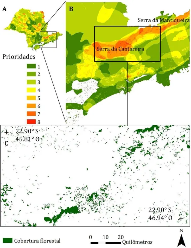
The study was conducted in the Cantareira-Mantiqueira region of the Atlantic Plateau of São Paulo state (Ponçano, 1981). The biodiversity conservation value of the Cantareira region has been formally recognized by the Environmental Ministry of Brazil (MMA, 2007).In addition the Cantareira-Mantiqueira region is responsible for almost 50% of the water supply of the city of São Paulo,

constituting one of the world’s largest urban water supply systems (Whately and Cunha, 2007). This region is covered with low montane evergreen forest and is characterized by rolling and steep convex hill with elevation ranging between 700 to 1700 m of altitude (N-S 22°50' - 23°26' and E-W 45°53'-46°46'; Fig. 2). This humid subtropical climate has dry winters and hot and humid summers, with annual rainfall that varies between 1350 and 2000 mm, and a mean annual temperature range of 15-22°C (www.cpa.unicamp.br). The approximately 26.3% of remaining forest in the region (IF, 2010) is classified as ombrophilous dense forest (IBGE, 2012) in different successional stages (Ditt et al., 2008; Ribeiro et al., 2009a; Teixeira et al., 2009), and is relegated to steep slopes of lower

land-use change, with much of the extensive cattle pasture area being further converted either into large-scale real estate development or incorporated into 'reforestation' projects, planted with Eucalyptus spp. (Fadini, 2005; Whately and Cunha, 2007).

2.2.Site selection and sampling design

Sample sites were selected in order to contrast edge ages (> 50 years vs < 50 years), and edge configurations (straight edges vs corner edges), but controlling forest fragment age (> 70 years). In order to select the studied fragments and sites, we first identified areas with land use and land cover changes that would potentially create edges with different ages. We considered available low resolution (pixel= 30 m) land use maps (1989, 1999, 2000, 2003 and 2010; Whately and Cunha, 2007; IF, 2010), and produced a temporal series of detailed land cover maps (1:5,000), using high resolution satellite images (SPOT and Digital Globe) and aerial photography (1:20,000-1:35,000) for the reference years 1962, 1978, 2003, 2007 and 2010. Considering the oldest forest fragments (the ones existing in the oldest available photograph of 1962 with a forest

structure), we looked for changes in border limits to determine different edge age classes. We were able to identify eight old-growth fragments (replicates) with two categories of border age (edges created before 1962, hereafter 'old' edges; and edges created after 1962, hereafter 'new' edges) and with the two categories of edge location (corner, and straight). Fragments ranged from 13 to 362 ha.

In each fragment, we placed five (n= 5) samples grouped into four treatments: fragment interior (n= 2); old corner edge(n= 1); old straight edge (n= 1); and new straight edge(n= 1)(Fig. 3). To be considered a straight edge, a site's sampling plot had to be at least 50 m far from corners. We avoided placing plots in slopes higher than 20 degrees, and attempted to standardize soil type to latosols - the predominant soil type in the region. Once matrix type can strongly modulate the impact of edge effects (Bender and Fahrig, 2005), we only

consisted of five circular plots with 10 m radius and center distant at least 20 m from one another. Edge plots were placed 5-40 m from the closest edge; interior plots were placed at least 110 m distant from every edge. All GIS analyses were conducted in ArcGIS 10 (ESRI, 2015).

2.3. Estimation of above ground biomass (AGB)

Measurements of aboveground carbon were conducted in April-September, 2014. In each circular plot, we measured the height and diameter at breast height (DBH) at 1.3 m from the ground of all trees, palms and ferns with DBH higher than 10 cm, including standing dead trees and palms.

We calculated aboveground biomass of individual trees using the allometric equation developed for secondary Atlantic forest by Burger and Delitti (2008):

= exp⁡ − . + . × ln × ℎ , (1)

where = tree above ground biomass (kg), = diameter at breast height (cm), and _ℎ = tree height (m).

Allometric equations for palms and ferns were provided by Hughes et al. (2013) and Tiepolo et al. (2002), respectively:

� = ��⁡ . × �� + . × . ⁄ ⁡⁡⁡⁡ (2)

= − ⁄ − × exp − . × ℎ , (3)

where _� = palms above ground biomass (kg), FB = tree ferns above ground biomass (kg).

Then, we calculated biomass per plot by the sum of individual biomass within each sampled plot, expressed as Mg ha-1_{. The conversion of AGB to carbon stock} follows Martinelli et al. (2000):

2.4. Response variables

Data on carbon stock density (Mg ha-1_{) were averaged across all plots to obtain} plot-level estimates. We separated this C stock into two tree size classes, grouped by tree DBH (i.e. small, 10- _{cm and larger cm to explore possible} differences in the proportion of DBH classes across different edge types. However, the small number of trees over 30 cm DBH prevented us from using this class as a response variable in the following analyses. Complementary to carbon stock, we utilized tree density, median tree height and basal area as response variables.

2.5.Explanatory variables

To evaluate the additive effects of edges, we used a model that considers the influence of all edges, as the integral of all edge effects within a predetermined distance from a focal point (Dmax) (Malcolm, 1994). We called this index the total edge effect index (EI). In the present study, we assume that the most intense effect on AGB loss due to edge effects occurs within 100 m from edges to the interior of the fragment (i.e. Dmax = 100 m). The model was implemented using the R package 'edgefx' (Goldberg and Ries, 2010) in the R statistical environment (R Core Team, 2014). We used our forest /non-forest classification map (year 2012) with 5 m pixel resolution, to generate raster images of edge density for each fragment (Fig. S1).

Besides edge age (> 50 years vs < 50 years) and position (straight edges vs corner edges), for each plot we considered an additional explanatory variable, the degree of human disturbance. To capture human disturbance across the study region, we adopted the disturbance or anthropogenic index (AI) proposed by Magalhães et al. (2015) . This index considers 14 indicators divided into three groups, with different weights in the final index score. Group 1 indicators

(weight=1) are those with implications for ecosystem simplification and local biodiversity loss, such as hunting or non-timber forest product extraction. Group 2 indicators (weight=1.5) are associated with ecosystem destruction or

Group 3 indicators (weight=2) have the potential to impact ecosystems in both manners, promoting biodiversity loss and ecosystem substitution (e.g. fire). The index ranges from 0 in areas without visible current human impact to 1 for fully impacted areas.

��⁡= �0⁄� × � (5)

�⁡ = ⁡ ∑ �� �⁄� (6)

Where ⁡�0 is the observed level of the indicator i, ⁡� is the maximum value of

each indicator, _� is the correspondent weight for each group and P is the sum of the weights of all indicators.

2.6.Statistical analysis

To test the hypothesis that edges will have lower C stock and smaller values of forest structure parameters (tree density, median tree height, basal area) than fragment interiors (hypothesis i), we built a linear mixed model of C stock as a function of plot position (edge or interior). Response variables for edge type comparisons were transformed in a ratio of edge plot type divided by the mean value of interior plots from the same fragment, in a paired approach. To test the effect of edge age (hypothesis ii) and edge position (hypothesis iii) on C stock and forest structure, we first fit C stock ratio as a function of edge age, EI and AI in a series of additive and interactive models. Additionally, we fitted other models using the ratio of basal area per plot, median height per plot and tree density per plot as response variables. For all models, we included fragment identity as a random effect, assuming that plots from the same fragment are expected to be more similar in comparison with plots from other fragments. We also included in model selection a null model with the response variable in function of a constant value. We selected the most plausible model using Akaike criterion Information (AIC), comparing the likelihoods of all candidate models.

We considered models with A)C as having substantial support evidence and

3. Results

General pattern

Across the eight fragments, we sampled a total of , stems cm DB( ,

comprising 3,006 stems in edge plots and 2,291 in interior plots. The total edge and interior plot areas sampled were 3.77 ha and 2.48 ha, respectively. The majority of sampled stems were trees (89%), followed by tree ferns (2.41%), palms (1.58%), and dead woody biomass (7.28%). For all plots, thin _DB( 30 cm) and short (height < 11 m) trees composed the majority of stems sampled, followed by medium trees (DBH 30 – 50 cm; height 11-16 m), while large

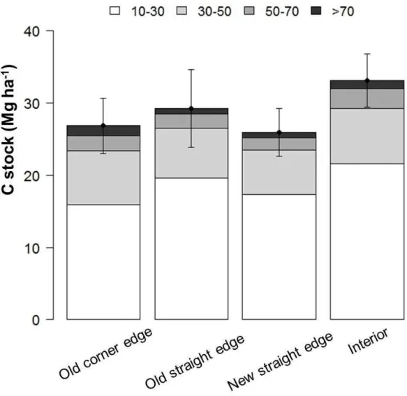
(DBH>50 cm) and tall trees 21 m height) were almost absent (Fig. 4A and 4B). C stock was highly variable between plots, ranging from 6.61 - 87.96 Mg, with a total average of 29.55 ± 14.97 Mg ha-1_{. Despite this variability, mean C stocks per} edge treatment were quite similar (Fig. 5), and only interior plots seems to be substantially different from edge treatments. Tree density per treatment shows a tendency to be in accordance with our predictions, with old corner edge having lower density, followed by old straight edges, new straight edges and interior treatment. Such trend does not seem to occur for basal area and median tree height, in which edge treatments have similar scores and interior treatments are slightly higher (Fig. S2A, S2B and S2C, respectively). We excluded tree ferns, palms, dead steams and one unusually large tree from all further analyses, as live trees were responsible for 99 % C pool.

Edge effects

The AIC top model for the contrast between interior and edge plots

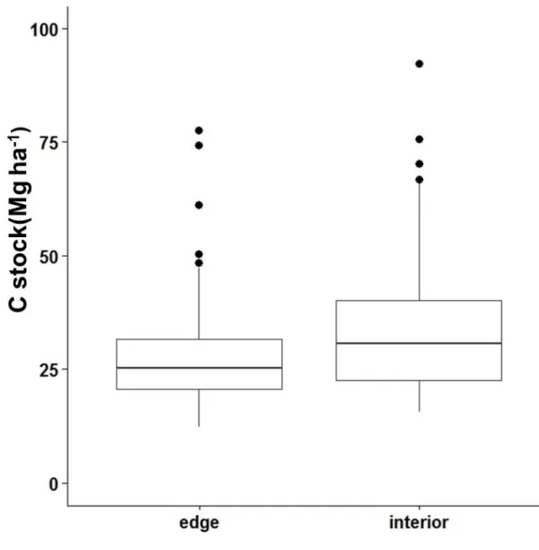
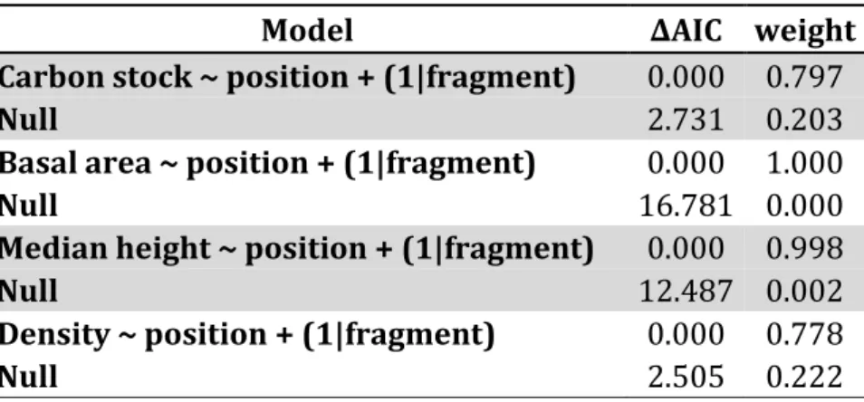
demonstrated that interior plots (mean=33.52 _± 16.81 Mg ha -1_{) have higher C} stock than edge plots (mean=27.51 _± 13.29 Mg ha -1_{) (Fig. 6), in accordance with} the first hypothesis. In fact, interior plots had higher tree density, basal area and median tree height (Table 1; Fig. S3, S4 and S5, respectively) in comparison with edge plots.

of 10-30 cm DBH, we did found that this class diameter composes a bigger

fraction of C pool in new edges, in comparison with old edges (Fig. 7). In addition, new edges have higher tree density than old edges (Fig. S6). Besides, for both new and old edges, tree density increases with the decrease of additive edge effects index (EI). For basal area and median height, we did not find any relation with edge effects (Table 2).

4. Discussion

We assessed the implications of edge effects for carbon stocks in a tropical forest disturbed and fragmented for a long time with a well-sampled dataset,

comprised of over 5,000 sampled stems within eight forest fragments considering additive edge effects and edge age. We corroborate our initial

hypothesis that interior forests have different tree structure than edge forests in Atlantic rainforest patches, with higher carbon stock, basal area, tree density and taller trees. However, contrary to our expectations, we found few differences in C stocks in edges with different ages and configurations, suggesting a distinct pattern of edge effect in those disturbed tropical landscapes.

Interior vs edges C stocks in disturbed tropical forests

The structural differences observed between edge (0-50 m) and interior (>100 m) were less pronounced than the clear patterns observed in the

Biological Dynamics of Forest Fragments Project (BDFFP), in the Amazon forest. This long-running project has provided the vast majority of theoretical and empirical work on tropical forest above-ground carbon response to

forest such as most fragments across the Atlantic forest fragments (Dean, 1996). In those old growth forests, edge effects are essentially related with the higher mortality of old trees, which concentrate most of above-ground carbon stocks (Stephenson et al., 2014). However, those old trees are largely absent from most secondary Atlantic forest fragments, even within fragment interiors,

considerably reducing the differences between interior and edges. Moreover, many human disturbances in the Amazon are relatively recent (e.g. from the early 1980s) and additional human disturbances such as major fires and logging were prevented in the BDFFP sites (Laurance et al., 2011). We suggest thus that the long history of human disturbance in the Atlantic forest creates a

heterogeneous mosaic of forest with different degrees and ages of disturbance, which may mask clearer differences between edges and interior areas.

Our results suggest thus that C stock in the Atlantic forest is widely affected by human disturbance and edge effects, creating a situation of low C stocks across the entire extent of remaining fragments, independent of edge distance, age or location. Indeed, previous studies in the Atlantic forest present evidence for strong reductions in AGB even into central areas of fragments up to 500 m from forest edges (de Paula et al., 2011). The same authors were only able to find a clear distinction between interior (defined as 200-1000 m) and edge plots for a very large (3,500 ha) reserve – where anthropogenic disturbances were

other tropical forests, such as the Amazonian forest, if present rates of deforestation persist for a long time.

While the overall small size and complex shapes of our forest fragments suggests that even our interior plots may be submitted to edge effects, we still found differences in tree size between interior and edge plots. Probably, two inter-related processes are acting to influence tree size. First, frequent and long-term disturbance may be retarding the regeneration process, resulting in a prevalence of small tree species and pioneers throughout fragments. Second, increased mortality due to edge effects tends to influence entire small forest fragments, though with higher intensity in the edges. Wind and abiotic factors such as aridity and higher temperatures (Murcia, 1995; Chen et al., 1999) cause structural changes in the forest, altering tree proportions and making stems shorter for a given basal DBH (Oliveira et al., 2008; de Paula et al., 2011). Oliveira et al. (2008) reported that trees were 30% shorter in edges when compared with edge-effect free areas in the Atlantic forest. In addition, the relaxing of

competition for light in edges might further reduce tree height for the same DBH (Osuri et al., 2014), as trees do not need to trespass the canopy to receive light. Consequently, trees in edge plots with the same DBH as interior plots tend to be a little smaller. In fact, observational(Feldpausch et al., 2011) and experimental (Holbrook and Putz, 1989) data shows thatboth plot density and shade can modulate tree H:DBH and, as a consequence, carbon stock.

It is important to highlight that although we expected to find contrasting differences in forest structure and above-ground carbon between fragment interiors and edges, there is remarkably little evidence to support this in the literature (Melito et al., submitted). One of the reasons raised to explain the lack of difference is related to tree density. Schedlbauer et al. (2007), for example, observed elevated tree density at forest edges, as well as higher AGB, and did not detect significant differences in forest structure or AGB along 350 m

forest edge and interior environments (Schedlbauer et al._{, 2007}). It is very probable that the same phenomenon has happened in forest patches from our study region and the elevated density at some forest edges created situations in which edge plots had higher AGB than interior plots, reducing general contrast between edges and interiors.

Edge age and additive effects

Initially we supposed that old edges would have accumulated more negative microclimate effects than new edges, and for this reason, they would have lower AGB than new edges. Likewise, we supposed that corner edges submitted to the effects of more than one edge would be more negatively affected by edges. However, results did not support these predictions suggesting that climatic-driven edge effects could be masked by anthropogenic disturbances, time since edges were submitted to those disturbances in sampled edges and retarded successional process.

Edges are subject to relatively higher intensity of microclimate changes, especially in terms of light regime and water balance (Kapos, 1989;

Williamslinera, 1990; Laurance and Yensen, 1991), which often results in high tree mortality (Lovejoy et al., 1986; Sizer and Tanner, 1999; Laurance et al., 2002; Numata et al., 2009). However, this overall biomass decay can occur rapidly, in the immediate few years after edge creation (Numata et al., 2009). Given that even our 'new' edges (< 50 years) would have already passed through this acute biomass decay stage, older edges may actually have relatively higher or similar AGB than new edges (an opposite effect than we predicted).

Compounding this loss of biomass in fragment edges, the increased exposure and improved access to forest edges by humans may drive the selective logging and removal of larger trees in both new and older edges.

Amazon, Alvira and Putz (2004) found that largest trees were the most affected by lianas and had more crown damage than trees without lianas. As the

fragments visited here were extensively disturbed by lianas and bamboos (37 % of all plots), at interior and edges areas, it is reasonable to suppose that physical damage imposed on trees might have contributed to the low density of larger trees, with subsequent impacts on C storage, independently of forest edge location or age.

Our results do not support as well the pattern of additive edge effects observed in the Amazonian forest (e.g. Malcolm, 1994; Laurance et al., 2007). The edge effect index (EI) was selected in an additive model with edge age, interacting with the anthropic index (AI), when we considered only small trees (Table 2). Areas under high rate of anthropic disturbance and closer to edges have a high proportion of small trees, particularly for new edges. It seems that beyond the occurrence of edge effects in the remnant forests, the study region is under very strong confounding effect of direct anthropogenic disturbance.

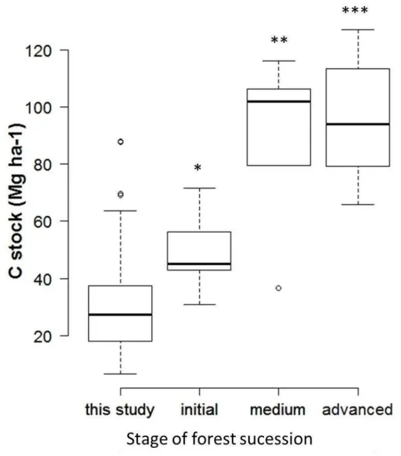
Additionally, previous studies variously suggest that secondary Atlantic forest may recover the structure of old growth forests after approximately 25–45 years (do Nascimento et al., 2014; Zanini et al., 2014), or much longer (Piotto et al., 2009). Even though all fragments visited have at least 70 years, the range of C stock values exhibited by edge and interior plots correspond to early (< 25 y old) or mid-successional secondary forest (25-45 yr old) (Figure 8. ). Indeed, we have clear evidence of a retarded successional process. For example, it is expected that large (DBH > 50 cm) and very large trees (DBH > 100 cm) play an important role in AGB pool for the Atlantic forest, similar to other Neotropical forests (DeWalt and Chave, 2004; Alves et al., 2010; Lindner, 2010). However, those size classes were almost absent from both interior and edge plots in this study (4A). Santos et al. (2008) suggested that these successional pathways may be crucially

homogeneity of forest structure and resultant carbon stocks between interior and edge areas, as we report previously.

Conservation implications

Tropical forests contain approximately one-third of terrestrial carbon pool (Dixon et al., 1994). Consequently, changes in C balance fluxes in tropical forest AGB have potentially important consequences on global C cycle, warming and biodiversity (Fearnside, 2004; Chave et al., 2005; Malhi, 2010), and accurate landscape measurements of C stocks are critical to generating a global view of the capacity of tropical forests to contribute to climate regulation. To date, published works are overly based on observations from the Amazon forest (Melito et al., submitted). Unfortunately, the Amazonian scenario may not be representative of most tropical forests in the near future, as human-modified forests are becoming the rule in the humid tropics (Achard et al., 2002; Melo et al., 2013; Haddad et al., 2015).

Differently from the Amazon forests, where edge effects have a clear and measurable influence in AGB and C stock, considering edge age and additive effects, such patterns are much less pronounced in human dominated landscapes, where long-history of disturbance greatly increases local

heterogeneity in forest structure. In those landscapes, remnant forest patches are in an early-to-middle-successional state and forest regeneration is not expected to result in late-successional or mature old-growth forests (Melo et al., 2013), at least without restoration.Our results of the carbon stock on early-stage and disturbed tropical forests have implications for improving our

understanding of the carbon storage potential of restored tropical forests.

Cantareira region, particularly, is very suitable for investment, as reforestation and degradation mitigation can greatly enhance carbon storage, water supply and biodiversity (Ditt et al., 2010; Shimamoto et al., 2014). With proper management, restoration projects have the potential to triple C stocks and enhance other ecosystem services.

Conclusions

We found no significant age or additive edge effects on carbon stocks in the studied Atlantic forest fragments. Structural differences between different edge types and even with interior areas were much less pronounced than the clear patterns observed for the Amazon forest. Besides, the carbon stock values we found are particularly low suggesting a significant effect of C loss by human disturbances in the fragmented Atlantic forest landscapes. Despite the difficulty to link historical disturbance with present forest structure, the legacy of past and present human impacts, with complex interactions, must play a fundamental role on determining spatial heterogeneity of tree community structure and dynamics in tropical forests. Our results suggest that much of unexplained variability in vegetation surveys in tropical forests could be related to the unique history of human use of each forest site.

5. Figures

6. Tables

Table 1. Candidate model sets following AIC model selection for the comparison between edge and interior treatments. We used as response variables carbon stock values per plot, basal area per plot, median tree height per plot and density per plot. The predictor variable Position indicates whether the plot is located in the interior (>110 m) or at the edge of the fragments sampled (5-40 m).

Model ∆AIC weight Carbon stock ~ position + (1|fragment) 0.000 0.797

Null 2.731 0.203

Basal area ~ position + (1|fragment) 0.000 1.000

Null 16.781 0.000

Median height ~ position + (1|fragment) 0.000 0.998

Null 12.487 0.002

Density ~ position + (1|fragment) 0.000 0.778

Table 2. Candidate model sets following AIC model selection for the comparison between edge treatments. We used as response variables the ratio of overall data on carbon stock values per plot (C); the ratio of the contribution of C stock in trees of 10-30 cm in relation to the total C stock (C10-30), the ratio of basal area

per plot, the ratio of median tree height per plot and the ratio of density per plot. Ratio values represent the contribution of each edge treatment plots in relation to interior plots (paired by fragment). We considered all models with _∆AIC _as equally plausible. Models coefficients are presented in Table S1.

Model ∆AIC Weight

Null 0 0.253

Ratio C ~ edge age + (1/fragment) 0.23 0.225

Ratio C ~ AI + edge age + (1/fragment) 1.431 0.124

Ratio C ~ edge age + EI + (1/fragment) 1.868 0.1

Ratio C ~ EI + (1/fragment) 1.994 0.093

Ratio C ~ AI+ edge age + EI + (1/fragment) 3.025 0.056

Ratio C ~ edge age + AI*EI + (1/fragment) 3.066 0.056

Ratio C ~ AI + edge age *EI + (1/fragment) 3.27 0.049

Ratio C ~ AI + EI + (1/fragment) 3.43 0.045

Ratio C10-30 + edge age + (1/fragment) 0 0.391

Ratio C10-30 ~ edge age + AI*EI + (1/fragment) 0.352 0.328

Ratio C10-30 ~ AI + edge age + (1/fragment) 0.914 0.211

Null 3.338 0.062

Ratio C10-30 ~ AI+ edge age + EI + (1/fragment) 3.587 0.055

Ratio C10-30 ~ AI + EI + (1/fragment) 5.397 0.022

Ratio C10-30 ~ edge age + EI + (1/fragment) 5.663 0.02

Ratio C10-30 ~ AI + edge age *EI + (1/fragment) 7.079 0.01

Ratio C10-30 ~ EI + (1/fragment) 7.753 0.007

Ratio density ~ edge age + EI + (1/fragment) 0 0.534

Ratio density ~ AI+ edge age + EI + (1/fragment) 1.923 0.204

Ratio density ~ edge age + AI*EI + (1/fragment) 3.461 0.095

Ratio density ~ AI + edge age *EI + (1/fragment) 3.575 0.089

Ratio density ~ edge age + (1/fragment) 4.323 0.061

Ratio density ~ EI + (1/fragment) 7.801 0.01

Ratio density ~ AI + EI + (1/fragment) 9.399 0.005

Null 18.17 0

Ratio density ~ AI + edge age + (1/fragment) 19.7 0

Null 0 0.285

Ratio basal area ~ EI + (1/fragment) 0.731 0.198

Ratio basal area ~ AI + edge age + (1/fragment) 1.332 0.146

Ratio basal area ~ edge age + (1/fragment) 1.825 0.114

Ratio basal area ~ AI + EI + (1/fragment) 2.183 0.096

Ratio basal area ~ edge age + EI + (1/fragment) 2.73 0.073

Model ∆AIC Weight Ratio basal area ~ edge age + AI*EI + (1/fragment) 4.67 0.028

Ratio basal area ~ AI + edge age *EI + (1/fragment) 4.825 0.025

Null 0 0.657

Ratio median height ~ AI + edge age + (1/fragment) 1.514 0.308

Ratio median height ~ edge age + (1/fragment) 7.611 0.015

Ratio median height ~ EI + (1/fragment) 7.795 0.013

Ratio median height ~ AI + EI + (1/fragment) 9.296 0.006

Ratio median height ~ edge age + EI + (1/fragment) 15.28 0

Ratio median height ~ edge age + AI*EI + (1/fragment) 16.26 0

Ratio median height ~ AI+ edge age + EI + (1/fragment) 16.76 0

Supporting Information

Table S1. Candidate model sets following AIC model selection for the comparison between edge treatments. Response variables for edge type comparison were transformed in a ratio of edge plot type divided by the mean value of interior plots from the same fragment, in a paired approach. (EI) - additive edge effect index; edge age - old or new; (AI) - index of anthropic disturbance. We have included fragment as a random variable.

Explantory

variables AI

edge

age EI edge age:EI AI:EI ∆AIC Weight

Ratio C

0 0.253

+ 0.23 0.225

1.031 1.431 0.124

+ 0.044 1.868 0.1

0.005 1.994 0.093

1.285 + 0.042 3.025 0.056

1.522 + 0.096 -3.769 3.066 0.056

1.27 + 0.28 + 3.27 0.049

1.03 0 3.43 0.045

Ratio C10-30

+ 0 0.391

1.952 + 0.035 -3.236 0.352 0.328

1.815 0.914 0.211

3.338 0.062

1.638 + 3.587 0.055

1.783 0.001 5.397 0.022

+ 0.069 5.663 0.02

1.659 + 0.002 7.079 0.01

0.08 + 7.753 0.007

Ratio density

+ 0.169 0 0.534

0.299 + 0.169 1.923 0.204

-0.146 + 0.149 2.218 3.461 0.095

0.291 + 0.229 + 3.575 0.089

+ 4.323 0.061

0.228 7.801 0.01

0.736 0.227 9.399 0.005

18.171 0

0.88 19.699 0

Ratio basal area

0 0.285

0.067 0.731 0.198

0.927 + 1.332 0.146

Explantory

variables AI

edge

age EI edge age:EI AI:EI ∆AIC Weight

0.83 + 0.063 2.183 0.096

+ 0.066 2.73 0.073

0.837 + 0.065 -3.038 4.18 0.035

1.183 + 0.103 4.67 0.028

0.836 + 0.213 + 4.825 0.025

Ratio median height

0 0.657

0.245 1.514 0.308

+ 7.611 0.015

-0.005 7.795 0.013

0.248 -0.005 9.296 0.006

+ -0.001 15.283 0

0.333 + 0.006 -0.802 16.256 0

0.256 + -0.001 16.756 0

Table S2. Published carbon (C) stock values from tropical forest inventories. We divided data into Atlantic Forest publications and other tropical forest publications. Sampling method, stage of forest succession, forest type and country where the inventory were done are presented when available. Inventory methodologies to sample stems and calculate C stocks are not standardized.

Sampling Stage of forest

sucessions Forest type Country Carbon stock Source Atlantic forest

Edge plots Initial Montane moist forest Brazil 27.28±13.18 This study

Edge transect Initial Montane moist forest Brazil 30.91±11 Romitteli (2014)

Edge plots Mature (protetected area) _{deciduous forest} Lowland semi- Brazil 42.1 Paula et al. (2011)

Fragment plots Initial Submontane moist _forest Brazil 42.89 Tiepolo et al. (2002)

Fragment plots Initial (protected area)

Lower montaine moist

forest Brazil 45.12

Groeneveld et al. (2009)

Fragment plots Initial Seasonal semideciduous

forest Brazil 56.31 Torres et al. (2013)

Fragment plots Initial Montane moist forest Brazil 71.6 Ditt et al. (2010)

Fragment plots Medium Seasonal semideciduous

forest Brazil 36.54 Souza (2011)

Fragment plots Medium Submontane moist

forest Brazil 101.96 Tiepolo et al. (2002)

Fragment plots Medium Atlantic moist forest Brazil 116.13 Burger (2005)

Fragment plots Medium/advanced Seasonal semideciduous

forest Brazil 79.38 Souza (2011)

Fragment plots Medium/advanced Submontane moist

Sampling Stage of forest

sucessions Forest type Country Carbon stock Source

Fragment plots Advanced (protetected

area)

Lower montane moist

forest Brazil 65.8

Groeneveld et al. (2009)

Fragment plots Advanced (protected

area)

Seasonally flooded

forest Brazil 72.996 Alves et al. (2010)

Fragment plots Advanced Atlantic moist forest Brazil 79.06 Cunha et al. (2009)

Fragment plots Advanced (protected _area) Lowland moist forest Brazil 94.04 Alves et al. (2010)

Fragment plots Advanced Montane moist forest Brazil 94 Vilela et al. (2012)

Fragment plots Advanced Montane moist forest Brazil 113 Vilela et al. (2000)

- Advanced Montane moist forest Brazil 113.43 Ditt et al. (2010)

Fragment plots Advanced Montane moist forest Brazil 127 Vilela et al. (2000)

Fragment plots Mature Seasonal semideciduous

forest Brazil 83.34

Ribeiro et al. ( 2009)

Fragment plots Mature (protetected area) Semideciduos seazonal _forest Brazil 108.98 ± 35.33 Amaro et al. (2013)

Fragment plots Mature (protected area) Submontane moist _forest Brazil 113.43 Alves et al. (2010)

Fragment plots Mature Submontane

ombrophilous forest Brazil 118.5±37.87

Lindner and Sattler (2012)

Sampling Stage of forest

sucessions Forest type Country Carbon stock Source

Fragment plots Mature (protetected area) Montane ombrophilous

forest Brazil 148.36 ±22.75

Lindner and Sattler (2012)

Fragment plots Mature Lowland semideciduous

forest Brazil 158.553 Rolim et al. (2005)

Fragment plots Mature (protetected area) Dense ombrophilous

forest Brazil 206.95 Lindner(2010)

Interior plots Initial Montane moist forest Brazil 33.24±16.7 This study

Interior plots Advanced (protetected

area)

Lower mountane moist

forest Brazil 117.5

Groeneveld et al. (2009)

Interior plots Mature (protetected area) Montane moist forest Brazil 124.52 Alves et al. (2010)

Other tropical forest

Edge transect Mature (protetected area) Tropical wet forest Costa Rica 170.3 ± 4.5 Schedlbauer et al.

(2007)

- Initial Lower montaine moist _forest Puerto Rico 53.1 Marin-Spiotta ₍₂₀₀₇₎ et al.

- Old growth Lower montane moist

forest Puerto Rico 103.9

Marin-Spiotta et al(2007)

- Old growth (protetected _area) Lowland moist forest Singapure 104.12 Ngo et al. (2013)

Mature (protetected area) Lowland moist forest Panama 84.89 DeWalt and Chave

(2004)

- Mature (protetected area) Lowland moist forest Singapure 111.21 Ngo et al. (2013)

Sampling Stage of forest

sucessions Forest type Country Carbon stock Source

Plots Mature (protetected area) Lowland moist forest Brazil 133.29 Vieira et al. (2004)

Plots Mature Lowland semideciduous

forest Brazil 138.45

Nascimento et al. (2007)

- Mature (protetected area) Central Amazonian Brazil 154.29 Nascimento and

Laurance (2002)

Conclusões gerais

Corroboramos nossa primeira hipótese ao constatar que o interior dos fragmentos possui uma estrutura florestal distinta das bordas, com maior

estoque de carbono acima do solo, maior área basal, maior densidade de árvores e árvores mais altas. Além disso, pudemos constatar que as bordas novas

possuem uma proporção maior de troncos finos (10 a 30 cm de diâmetro a altura do peito) compondo o estoque de carbono. Esta classe de diâmetro também apresentou maior densidade de indivíduos nas bordas novas. Entretanto, não encontramos diferenças em termos de estoque de carbono comparando os diferentes tipos de borda, tanto em relação à idade como a efeitos aditivos de borda analisando a totalidade dos dados. Deste modo, refutamos as hipóteses iniciais nas quais esperávamos encontrar maior estoque de carbono em bordas velhas e em bordas em quinas, respectivamente.Além disso, os valores de

estoque de carbono que encontramos foram surpreendentemente baixos, dentre os menores publicados para a Mata Atlântica.

Apesar de termos detectado diferenças na estrutura florestal entre o interior e as bordas dos fragmentos, mesmo considerando distâncias relativamente curtas, estas diferenças são menos pronunciadas do que os padrões claros já descritos para a floresta Amazônica. Esses dados sugerem que o padrão observado na Amazônia (Laurance et al., 2011) não deve ser utilizado como modelo de estudos para outras paisagens tropicais, em particular aquelas que têm um longo

histórico de fragmentação e perturbação, como as da Mata Atlântica. Nossos resultados demonstram que incorporar efeitos de borda nos modelos para extrapolação de estoques de carbono é algo complexo e que a alta

heterogeneidade local deve gerar imprecisões em estimativas de larga escala.

Uma diferença essencial entre a região Amazônica e a Mata Atlântica está ligada ao histórico de distúrbios antrópicos. A Mata Atlântica, desde o início da

colonização portuguesa, sofreu um intenso processo de destruição e degradação florestal (Dean, 1996), o que ainda não ocorreu nas áreas investigadas na