<sup>10</sup>Be in last deglacial climate simulated by ECHAM5-HAM – Part 1: Climatological influences on <sup>10</sup>Be deposition

(1)

CPD

9, 3681–3709, 2013

10_{Be in deglaciation –}

Part 1: Climatological influence U. Heikkilä et al.

Title Page

Abstract Introduction

Conclusions References

Tables Figures

◭ ◮

Back Close

Full Screen / Esc

Printer-friendly Version

Interactive Discussion

Discussion

P

a

per

|

D

iscussion

P

a

per

|

Discussion

P

a

per

|

Discuss

ion

P

a

per

|

Clim. Past Discuss., 9, 3681–3709, 2013 www.clim-past-discuss.net/9/3681/2013/ doi:10.5194/cpd-9-3681-2013

Open Access

Climate of the Past

Discussions

Geoscientiic Geoscientiic

This discussion paper is/has been under review for the journal Climate of the Past (CP). Please refer to the corresponding final paper in CP if available.

10

_{Be in last deglacial climate simulated by}

ECHAM5-HAM – Part 1: Climatological

influences on

10

Be deposition

U. Heikkilä1, S. J. Phipps2, and A. M. Smith1

1

Institute for Environmental Research, Australian Nuclear Science and Technology Organisation (ANSTO), Lucas Heights, NSW, Australia

2

ARC Centre of Excellence for Climate System Science and Climate Change Research Centre, University of New South Wales, Sydney, Australia

Received: 12 June 2013 – Accepted: 25 June 2013 – Published: 2 July 2013

Correspondence to: U. Heikkilä (ulla@ansto.gov.au)

(2)

CPD

9, 3681–3709, 2013

Title Page

Tables Figures

◭ ◮

Back Close

Full Screen / Esc

Discussion

P

a

per

|

D

iscussion

P

a

per

|

Discussion

P

a

per

|

Discuss

ion

P

a

per

|

Abstract

Reconstruction of solar irradiance has only been possible for the Holocene so far. Dur-ing the last deglaciation two solar proxies (10Be and14C) deviate strongly, both of them being influenced by climatic changes in a diff_{erent way. This work addresses the climate}

influence on10Be deposition by means of ECHAM5-HAM atmospheric aerosol-climate 5

model simulations, forced by sea surface temperatures and sea ice extent created by the coupled climate system model CSIRO Mk3L. Three time slice simulations were per-formed during the last deglaciation: 10 000 BP (“10k”), 11 000 BP (“11k”) and 12 000 BP (“12k”), each 30 yr long. The same10Be production rate was used in each simulation to isolate the impact of climate on 10Be deposition. The changes are found to follow 10

roughly the reduction in the greenhouse gas concentrations within the simulations. The 10k and 11k simulations produce a surface cooling which is symmetrically amplified in the 12k simulation. The precipitation rate is only slightly reduced at high latitudes, but there is a northward shift in the polar jet in the Northern Hemisphere and the strato-spheric westerly winds are significantly weakened. These changes occur where the 15

sea ice change is largest in the deglaciation simulations. This leads to a longer resi-dence time of10Be in the stratosphere by 30 (10k and 11 k) to 80 (12k) days, heavily increasing the atmospheric concentrations. Furthermore the shift of westerlies in the troposphere leads to an increase of tropospheric 10Be concentrations, especially at high latitudes. The contribution of dry deposition generally increases, but decreases 20

where sea ice changes are largest. In total, the 10Be deposition rate changes by no more than 20 % at mid- to high latitudes, but by up to 50 % in the tropics. We conclude that on “long” time scales (a year to a few years), climatic influences on10Be deposition remain small even though atmospheric concentrations can vary significantly. Averaged over a longer period all10Be produced has to be deposited by mass conservation. This 25

(3)

CPD

9, 3681–3709, 2013

Title Page

Tables Figures

◭ ◮

Back Close

Full Screen / Esc

Discussion

P

a

per

|

D

iscussion

P

a

per

|

Discussion

P

a

per

|

Discuss

ion

P

a

per

|

on10Be in terms of preserving the solar signal locally is analysed in an accompanying paper (Heikkilä et al., 2013).

1 Introduction

Cosmogenic radionuclides, such as10Be and14C, are commonly used proxies for solar activity. Their production rate in the atmosphere responds to changes in cosmic ray 5

intensity, which again is modulated by solar activity and the strength of the geomagnetic field. Their transport from the source to natural archives is subject to climatological modulation: atmospheric circulation and precipitation in the case of10Be and reservoir exchange times in the case of 14C. Comparison of both radionuclides allows for the separation of the common production, or solar, signal from the climate modulation. 10

Recent results show that during the Holocene the climate impact remains relatively small and the solar signal can be retrieved (e.g. Steinhilber et al., 2012). However, extending the solar forcing function into the last deglaciation becomes challenging as large discrepancies arise between 14C and 10Be (e.g. Muscheler et al., 2004). The reason for these diff_{erences has to be understood before the solar forcing function can}

15

reliably be extended to this period.

In order to address the sensitivity of 10Be deposition onto polar ice sheets to cli-mate changes we perform time slice simulations within the deglacial clicli-mate at three diff_{erent stages: 12 000 BP (years before 1950 CE), 11 000 BP and 10 000 BP. A}

prein-dustrial control simulation is also performed for comparison. These simulations are 20

referred to as “ctrl”, “12k”, “11k” and “10k” throughout the manuscript. The model em-ployed is the ECHAM5-HAM chemistry-transport model. This incorporates the aerosol module HAM, which describes aerosol emission, physical and chemical as well as de-position processes. This model only describes the atmosphere and hence requires the sea surface temperatures and sea ice cover to be described. In this study these vari-25

(4)

CPD

9, 3681–3709, 2013

Title Page

Tables Figures

◭ ◮

Back Close

Full Screen / Esc

Discussion

P

a

per

|

D

iscussion

P

a

per

|

Discussion

P

a

per

|

Discuss

ion

P

a

per

|

2012). ECHAM5-HAM resolves aerosol processes explicitly. This is important in order to obtain a realistic picture of aerosol deposition and its climate modulation, but at the same time it increases the runtime of the model. Such a time-slice approach focusing on periods of special interest, such as the Last Glacial Maximum or the mid-Holocene, is commonly used in model intercomparison experiments (e.g. Braconnot et al., 2012), 5

or when addressing questions such as atmospheric particle transport under a changing climate (e.g. Krinner et al., 2010; Mahowald et al., 2006).

The focus of this study is to investigate the impact of the deglacial climate on10Be deposition. The reconstructing of the solar signal from the10Be deposition rate during this period is addressed in an accompanying paper (Heikkilä et al., 2013). In order to 10

be able to distinguish the imprint of climate only, and also because the actual solar activity and therefore the10Be production rate are unknown, we use the same (theo-retical) production rate in all simulations. This means that even if the model climate in each time slice simulation is quite diff_{erent, the global mean}10_{Be deposition rate will}

be equal due to mass conservation. Because of this a direct comparison with mea-15

sured10Be concentrations is not possible. In terms of climate these time slice simu-lations produce typical climatic conditions given the boundary conditions determined by greenhouse gas concentrations (GHGs), orbital parameters and aerosol load. The internal climate variability produced by the model will be representative in a statistical sense under these boundary conditions, although the actual timing and magnitude of 20

individual weather events will not be reproduced.

Comparison of10Be and14C during the Younger Dryas has previously been used to detect changes in North Atlantic deep-water formation and the carbon cycle (Muscheler et al., 2000, 2004): however, both10Be and14C are influenced diff_{erently by changes}

in climatic conditions which hampers the detection of the common solar signal. To the 25

(5)

CPD

9, 3681–3709, 2013

Title Page

Tables Figures

◭ ◮

Back Close

Full Screen / Esc

Discussion

P

a

per

|

D

iscussion

P

a

per

|

Discussion

P

a

per

|

Discuss

ion

P

a

per

|

2 Description of the simulations

Boundary conditions for the ECHAM5-HAM simulations were obtained from simula-tions of the pre-industrial ctrl, 10k, 11k and 12k climate conducted using the CSIRO Mk3L climate system model. This is a coupled general circulation model, consisting of components that describe the atmosphere, land, sea ice and ocean (Phipps et al., 5

2011, 2012). The model was integrated for 5000 yr in each case to let the system reach thermal equilibrium and the last 35 yr were then used to provide boundary conditions for the ECHAM5-HAM simulations of the atmosphere. For each time slice simulation, the CSIRO Mk3L simulations used constant orbital parameters and greenhouse gas concentrations (obtained from Liu et al., 2009, see Table 1). The total solar irradiance 10

was held fixed at 1365 W m−2

in each experiment. Land ice extents were prescribed according to the ICE-5G reconstruction v1.2 (Peltier, 2004). No changes were made to global sea level or to the positions of the coastlines.

The ECHAM5-HAM atmospheric model used sea surface temperatures (SST) and sea ice cover generated by the CSIRO Mk3L model as ocean boundary conditions. 15

The greenhouse gas concentrations, orbital parameters, orography and land sea mask were set to the same values as in the CSIRO Mk3L simulations according to the PMIP2 protocol (http://pmip2.lsce.ipsl.fr/). The SSTs and sea ice were updated monthly. Aerosol load was set to preindustrial values for the simulations and was taken from the AEROCOM aerosol model-intercomparison experiment B, available at 20

http://nansen.ipsl.jussieu.fr/AEROCOM. The ECHAM5-HAM model was run for 35 yr, from which the first 5 yr were used to spin up the model and discarded. The hori-zontal resolution used was the T42 spectral resolution, corresponding to ca. 2.8◦

or ca. 300 km. The model top was at ca. 30 km, including 31 vertical levels. The model output was analysed monthly. In order to analyse the atmospheric transport path of 25

10

(6)

CPD

9, 3681–3709, 2013

Title Page

Tables Figures

◭ ◮

Back Close

Full Screen / Esc

Discussion

P

a

per

|

D

iscussion

P

a

per

|

Discussion

P

a

per

|

Discuss

ion

P

a

per

|

for a more realistic particle transport towards the poles following Bourgeois and Bey (2011).

The 10Be production rate on the monthly scale was constructed using a low-frequency solar activity parameterΦ _{based on a reconstruction of the}14_{C production}

rate, and a modern 11 yr cycle was added on top. This leads to a 10Be production 5

rate which is ca. 70 % larger than typical values during the last ca. 30 yr (see for ex. Heikkilä and Smith, 2012).

3 Results

3.1 Global means and budgets

Table 1 summarises the global mean temperatures and precipitation rates over each 10

30 yr period. It is clear from the results that the global mean temperature closely fol-lows the GHGs. The GHGs during 10k and 11k are fairly similar, leading to a cooling of ca. 1◦

from ctrl. The 12k simulation is cooler, 2.7◦

relative to ctrl, due to a larger reduction of the GHGs. These diff_{erences are somewhat larger than the 0.6}◦ _global cooling during the Younger Dryas (12.9 to 11.7 ka BP) reported by Shakun and Carl-15

son (2010). An explicit comparison is hard because the model simulations present two 30 yr snapshots during this period. Shakun and Carlson (2010) analysed all available proxy data worldwide but large areas, especially oceans, are still uncovered. Because of this their global mean change would be milder if ocean temperatures were given more weight. However, the model simulations presented here have been fully equilibri-20

ated, and hence the magnitude of the cooling might exceed the transient response of the climate system.

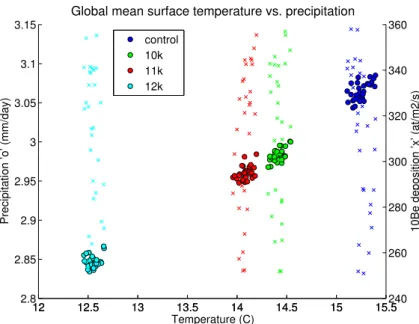
The precipitation rate varies less between the simulations, however a linear response to cooling, albeit a weak one, is evident (Fig. 1). Table 2 summarises the global mean

10

Be budgets over each 30 yr period. The ctrl simulation produces results consistent 25

(7)

CPD

9, 3681–3709, 2013

Title Page

Tables Figures

◭ ◮

Back Close

Full Screen / Esc

Discussion

P

a

per

|

D

iscussion

P

a

per

|

Discussion

P

a

per

|

Discuss

ion

P

a

per

|

the stratosphere, and the residence time is of the order of one year in the stratosphere and ca. three weeks in the troposphere (e.g. Heikkilä and Smith, 2012; Koch et al., 2006; Land and Feichter, 2003). The total contents of 10Be in the stratosphere and the troposphere in these simulations are slightly larger than modern values due to the higher production rate.

5

During the deglaciation the stratospheric fraction of production is slightly increased due to a lower tropopause height. Again, this change is larger during 12k than 10k and 11k. Moreover, the fraction of wet to total deposition is decreased to 87–88 % in all simulations, which is a reduction relative to the typical simulated present-day value of 91–92 % produced by this model (Heikkilä et al., 2009). The stratospheric and 10

tropospheric residence times are both increased, leading to higher atmospheric10Be contents. This is likely to be due to circulation changes which will be discussed in the following section.

3.2 Changes in atmospheric circulation

We first investigate the general state of climate in the deglaciation simulations com-15

pared with the control climate. Figure 2 shows the zonal mean temperature change relative to ctrl in all simulations. The 10k and 11k simulations show a moderate cooling in the tropical upper troposphere and a warming of the stratosphere. The cooling is slightly increased in the 11k simulation, including a cooler region in the northern high latitude lower levels. This pattern is intensified in the 12k results with the 50–90◦_N 20

lower level cooling becoming stronger. A surface cooling and stratospheric warming in response to reduced atmospheric GHGs is consistent with the nature of the observed response to increased GHGs during the 20th century (Trenberth et al., 2007). Zonal mean westerly winds (Fig. 3) show a similar response: a slight weakening of the SH mid-latitude and NH low latitude stratospheric winds and a slight intensification in the 25

(8)

CPD

9, 3681–3709, 2013

Title Page

Tables Figures

◭ ◮

Back Close

Full Screen / Esc

Discussion

P

a

per

|

D

iscussion

P

a

per

|

Discussion

P

a

per

|

Discuss

ion

P

a

per

|

to a slower circulation and hence less effi_{cient particle transport, causing the}

strato-spheric residence time of10Be to increase (Table 1).

The shift found in the NH tropospheric westerlies can possibly be connected to the position of storm tracks and therefore to precipitation patterns. However, no such shift is obvious in the precipitation rate (Fig. 4), nor in the sea level pressure (not shown). 5

There is a general decrease in the simulated precipitation rate in the mid- and high latitudes (both NH and SH), in agreement with the cooling caused by the lower GHG concentrations (see Fig. 1). At low latitudes, however, there is an increase in precipita-tion of up to 50 %, mostly in dry areas (Sahara, west of the South American and African continents). In order to study the intensity of internal climate variability we performed 10

an EOF analysis for the sea level pressure. The first EOF of SLP (associated with NAO in the North Atlantic sector and SAM south of 20◦ _{in the SH, Fig. 5) does not exhibit} significantly larger variability in the deglaciation simulations than in the control, sug-gesting that the internal climate variability described by these modes did not change significantly.

15

The diff_{erences between the simulations seem fairly symmetric except for the shift of}

the zonal wind in the NH troposphere poleward of 50◦_{. The reason for this asymmetry} might be the larger sea ice content in the deglaciation simulations, especially in the NH (Fig. 6). Sea ice conditions influence atmospheric circulation patterns, such as sea level pressure, strength of the westerlies and position of the storm tracks, in the 20

northern mid- and low latitudes and even globally via teleconnections aff_ecting

large-scale circulation patterns such as ENSO (e.g. Alexander et al., 2004; Blüthgen et al., 2012; Budikova, 2009; Screen and Simmonds, 2010). However, we find a decrease in geopotential height at the surface where the sea ice increase is largest, both in the NH and the SH, although the anomaly is visible at 500 hPa only in the NH. Thus the 25

1000–500 hPa thickness is reduced in the deglaciation simulations due to increased sea ice. The reduction is largest near the Hudson Bay area where sea ice diff_erences

(9)

CPD

9, 3681–3709, 2013

Title Page

Tables Figures

◭ ◮

Back Close

Full Screen / Esc

Discussion

P

a

per

|

D

iscussion

P

a

per

|

Discussion

P

a

per

|

Discuss

ion

P

a

per

|

tropopause height is seen at 35◦_{N. This suggests that the anomalous NH temperature,} shift in the westerlies and longer atmospheric residence time of10Be are resulting from the increased sea ice in the deglaciation simulations.

3.3 Circulation influence on atmospheric distribution of10Be

The changes found in climatic conditions of the deglaciation simulations, the weaken-5

ing of the stratospheric jets, the northward shift in the westerlies and the changes in tropopause height all have the potential to aff_{ect particle transport and deposition and}

hence 10Be. In the following we investigate the modelled changes in 10Be between the deglaciation simulations and the control climate. Firstly we investigate whether the general relationship between GHGs, surface temperature and precipitation rate could 10

be used to predict the 10Be deposition under diff_{erent climatic conditions. In addition}

to temperature and precipitation, Fig. 1 shows the global and annual mean10Be depo-sition flux (crosses) as a function of mean surface temperature for each year of each simulation. No relationship between global mean temperature and10Be deposition is obvious because the amplitude of the 11 yr cycle dominates the changes in tempera-15

ture or precipitation rate. If averaged over the entire 30 yr period the10Be deposition change is zero, as determined by the fact that the production rate is the same. Hence, a simple linear relationship between mean climate and 10Be deposition can not be assumed.

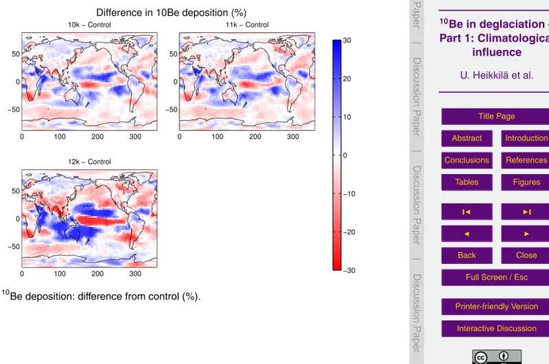
Figure 7 illustrates the mean change in10Be deposition flux. Because the production 20

rate of 10Be was the same in all simulations the global mean change equals zero.

10

Be deposition is not significantly changed at mid to high latitudes in the 10k and 11k simulations. It is increased in the NH over Siberia and Greenland, with the exception of Scandinavia and the Hudson Bay area, where changes in sea ice extent are largest. In the SH the 10Be deposition is decreased over the Southern Ocean but generally 25

increased over Antarctica. The change in deposition is larger in the tropical region and its sign varies. Then the diff_{erence in deposition in the 12k simulation is similarly}

(10)

CPD

9, 3681–3709, 2013

Title Page

Tables Figures

◭ ◮

Back Close

Full Screen / Esc

Discussion

P

a

per

|

D

iscussion

P

a

per

|

Discussion

P

a

per

|

Discuss

ion

P

a

per

|

latitudes. However, the simulated change at 12k becomes negative over North America whereas it is slightly positive at 10k and 11k. Over Greenland the deposition increases less at 12k than at 10k or 11k.

The changes in10Be deposition partly follow the precipitation change, especially in the tropics. Also the positive change over Greenland and the negative one over Scandi-5

navia and the Hudson Bay area are consistent with the precipitation change. However, the precipitation changes at 12k are larger than at 11k or 10k which is not seen in the

10

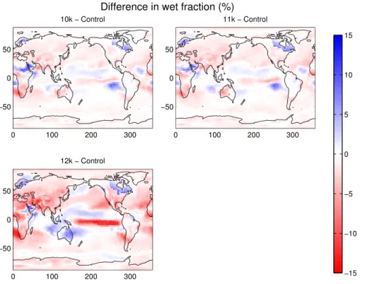
Be deposition change, and the strongly negative precipitation change at 12k over North America does not correspond to the 10Be deposition increase there. Table 1 shows that the global mean fraction of wet to total10Be deposition is similar in all sim-10

ulations, however it is reduced from the present day value of 91–92 % (Heikkilä et al., 2009). Figure 8 shows the spatial distribution of the change in wet fraction relative to ctrl. The change is small but roughly follows the precipitation change. In Scandinavia and the Hudson Bay area the wet fraction is increased instead of decreased although the10Be deposition is decreased, suggesting a dilution eff_{ect. In Greenland, where the}

15

deposition change diff_{ers from the surrounding areas, no change is apparent in the}

wet fraction. In total the wet fraction change remains small (up to 15 %) but locally the dry deposition and sedimentation increase by over 50 %. However, wet deposition re-mains the dominant method of removal of10Be from the atmosphere. To summarise, the10Be deposition diff_{erences globally are due to a combination of precipitation and}

20

atmospheric circulation changes, triggered by the increase in sea ice extent.

The circulation changes at mid- and high latitudes largely aff_{ect particle transport}

and dry deposition, which causes the air concentration of 10Be to increase (Fig. 9). The largest increase in concentrations is found in the tropical tropopause region, in-dicating a weaker stratospheric transport. Outside of these regions there is a rather 25

(11)

strato-CPD

9, 3681–3709, 2013

Title Page

Tables Figures

◭ ◮

Back Close

Full Screen / Esc

Discussion

P

a

per

|

D

iscussion

P

a

per

|

Discussion

P

a

per

|

Discuss

ion

P

a

per

|

sphere. These changes follow the pattern of change of age of air between the simula-tions, derived from the modelled10Be/7Be ratios (Fig. 10).10Be and7Be are produced in a near-constant ratio (gradually decreasing from 0.3 at ca. 30 km altitude to 0.8 near the surface, Heikkilä et al., 2008) which increases because7Be decays with its half-life of 53.2 days. The largely increased age of air in the stratosphere is consistent with the 5

reduced strength of stratospheric zonal winds (Fig. 3). The diff_{erences are smallest at}

high latitudes where the production of new10Be and7Be decreases the mean ratio. These changes in atmospheric circulation, 10Be air concentrations and transport path of10Be from source to archive can potentially influence the mixture of10Be from diff_{erent atmospheric source regions in deposition. The} 10_{Be production varies by}

or-10

ders of magnitude across latitude and altitude. Furthermore, the production is more strongly modulated by varying solar activity at high latitudes and altitudes, where it is highest to begin with. Therefore, a change in source-to-archive atmospheric transport path of10Be could lead to a catchment of10Be from a production area reflecting solar activity with a diff_{erent amplitude from the global mean production. Figure 11 illustrates}

15

the source-to-archive distribution of10Be for each of the simulations. The general dis-tribution in these simulations is very similar to the previously studied present day sit-uations (Heikkilä and Smith, 2012, their Fig. 12): 10Be produced in the stratosphere is mainly transported into the troposphere via the mid-latitudes and deposited equally between the 0–30◦ _{and 30–60}◦ _{latitude bands in each hemisphere. The tropospheric} 20

production of10Be is mostly deposited locally and the neighbouring latitude bands and rarely makes it to the opposite hemisphere. The figure shows that the diff_erences

be-tween the control simulation and the deglaciation simulations are fairly small. In the SH the production and deposition distribution is practically unaff_{ected by climatic changes}

in these simulations. The circulation change can be seen in latitude bands 30–60◦_N 25

(12)

tropo-CPD

9, 3681–3709, 2013

Title Page

Tables Figures

◭ ◮

Back Close

Full Screen / Esc

Discussion

P

a

per

|

D

iscussion

P

a

per

|

Discussion

P

a

per

|

Discuss

ion

P

a

per

|

sphere. The stratospheric production of10Be (ca. 2/3 of total), which is also the most heavily modulated, is unaff_{ected by the deglacial climate. The fairly large di}ff_{erences in}

atmospheric circulation found within the 10k, 11k and 12k simulations do not influence

10

Be transport as much as between the control and any of the deglaciation simulations. These diff_{erences are comparable in amplitude with those caused by di}ff_{erent model}

5

resolutions or realisations in Heikkilä and Smith (2012).

4 Summary and conclusions

This study investigates climatic influences on10Be deposition during the last deglacial climate. Three time slice simulations were performed, each of 30 yr duration: 10 000 BP (10k), 11 000 BP (11k) and 12 000 BP (12k). These simulations were compared with 10

a control (ctrl) simulation representing the preindustrial climate. The model employed was the atmospheric ECHAM5-HAM aerosol-climate model, driven by sea surface tem-peratures and sea ice cover produced by the coupled atmosphere-ocean-sea ice-land surface model CSIRO Mk3L. This paper, presenting the first part of this study, focuses on changes in atmospheric mean circulation and climate and their impact on the at-15

mospheric distribution and deposition of10Be. The second part (Heikkilä et al., 2013) investigates the influence of deglacial climate on10Be deposition in terms of preserv-ing the solar signal. In order to separate the pure climate modulation of10Be, and also because the solar activity during the deglaciation is not known, the 10Be production was kept the same in all simulations. Hence the results are not suited for comparison 20

with actual observations.

Generally the results follow changes in the greenhouse gas concentrations. Surface temperatures are colder and the precipitation rate reduced in the 10k and 11k simu-lations from ctrl, and these diff_{erences are amplified in the 12k simulation. Similarly,}

stratospheric zonal winds are weakened in the 10k and 11k simulations, and more 25

(13)

CPD

9, 3681–3709, 2013

Title Page

Tables Figures

◭ ◮

Back Close

Full Screen / Esc

Discussion

P

a

per

|

D

iscussion

P

a

per

|

Discussion

P

a

per

|

Discuss

ion

P

a

per

|

locally in Scandinavia and the Hudson Bay area, leading to a decreased 10Be de-position in these areas although the10Be deposition is generally decreased at mid-and high latitudes. Sea ice changes increase the fraction of wet deposition to total as opposed to the surrounding areas where dry deposition is increased due to reduced the precipitation rate. The reduced stratospheric winds lead to a reduced10Be trans-5

port, increasing the stratospheric residence time by 30 (10k and 11k) to 80 (12k) days. Tropospheric residence time is also increased by a few days, mainly at mid- to high lat-itudes due to the circulation changes. Atmospheric concentrations of10Be are strongly increased (>50 %) in the upper troposphere at mid- to high latitudes and in the tropical tropopause region. These circulation changes seem to be attributed to the increase 10

in sea ice extent in the deglaciation simulations, leading to anomalies in geopoten-tial height and shifts in position of the polar jet. In the Southern Hemisphere (SH) the disturbances due to increased sea ice are only evident near the surface.

Despite the changes found in atmospheric circulation and the regionally varying re-sponse of10Be air concentrations the source-to-archive distribution is fairly similar in 15

all simulations. The largest change was found in the NH polar troposphere due to the reduced10Be deposition, leading to up to 8 % less deposition of locally produced10Be, compensated by an increase of 0–30◦_N 10_{Be. Most of} 10_{Be produced in the} strato-sphere is deposited between 60◦

S and 60◦

N, uninfluenced by the deglacial climate. Generally the longer residence time in the deglaciation experiments allows for slightly 20

increased long-range tropospheric transport in the NH. Due to the longer stratospheric residence time the mixing of the large production gradients of 10Be along latitude is more thorough.

These results indicate that10Be deposition is mostly determined by mass balance. If the production rate does not change, the global mean deposition change will be zero. 25

(14)

CPD

9, 3681–3709, 2013

Title Page

Tables Figures

◭ ◮

Back Close

Full Screen / Esc

Discussion

P

a

per

|

D

iscussion

P

a

per

|

Discussion

P

a

per

|

Discuss

ion

P

a

per

|

aff_{ect the atmospheric residence time (80 days at most in these experiments) leading}

to a later deposition and a more thorough mixing of 10Be. However, averaged over a few years, this eff_{ect is smoothed out. In fact the longer residence time in colder}

climates leads to an increased mixing of10Be in the atmosphere and therefore a more homogeneous deposition pattern. Combining all these changes the total deposition 5

change was maximally 50 %. This is in agreement with the results of Alley et al. (1995), who found only moderate changes in10Be during the Younger Dryas.

Given these results,10Be deposition flux would be the optimal proxy for solar activity in an ideal archive because, following mass balance, the atmospheric production of

10

Be will have to be deposited at the surface within a few years. In case of10Be snow 10

concentrations the mass balance does not necessarily hold due to potential changes in precipitation rate. In reality, however, the10Be deposition flux has to be derived from the reconstructed snow accumulation rate which adds some uncertainty to the record.

Acknowledgements. This work was supported by an award under the Merit Allocation Scheme on the NCI National Facility at the ANU.

15

References

Alexander, M. A., Bhatt, U. S., Walsh, J. E., Timlin, M. S., Miller, J. S., and Scott, J. S.: The atmospheric response to realistic arctic sea ice anomalies in an AGCM during winter, J. Climate, 17, 890–905. 3688

Alley, R. B., Finkel, R. C., Nishiizumi, K., Anandakrishnan, S., Shuman, C. A., Mershon, G., 20

Zielinski, G. A., and Mayewski, P. A.: Changes in continental and sea-salt atmospheric load-ings in central Greenland during the most recent deglaciation: model-based estimates, J. Glaciol., 41, 139, 503–514, 1995. 3694

Blüthgen, J., Gerdes, R., and Werner, M.: Atmospheric response to the extreme Arctic sea ice conditions, Geophys. Res. Lett., 39, L02707, doi:10.1029/2011GL05486, 2012. 3688 25

(15)

CPD

9, 3681–3709, 2013

Title Page

Tables Figures

◭ ◮

Back Close

Full Screen / Esc

Discussion

P

a

per

|

D

iscussion

P

a

per

|

Discussion

P

a

per

|

Discuss

ion

P

a

per

|

Braconnot, P., Harrison, S. P., Kageyama, M., Bartlein, P. J., Masson-Delmotte, V., Abe-Ouchi, A., Otto-Bliesner, B., and Zhao, Y.: Evaluation of climate models using palaeoclimatic data, Nature Climate Change, 2, 417–424, doi:10.1038/nclimate1456, 2012. 3684

Budikova, D.: Role of Arctic sea ice in global atmospheric circulation: a review, Global Planet. Change, 68, 149–163, doi:10.1016/j.gloplacha.2009.04.001, 2009. 3688

5

Heikkilä, U. and Smith, A. M.: Influence of model resolution on the atmospheric transport of

10

Be, Atmos. Chem. Phys., 12, 10601–10612, doi:10.5194/acp-12-10601-2012, 2012. 3685, 3686, 3687, 3691, 3692

Heikkilä, U., Beer, J., and Alfimov, V. A.: Beryllium-10 and beryllium-7 in precipitation in Düben-dorf (440 m) and at Jungfraujoch (3580 m), Switzerland (1998–2005), J. Geophys. Res., 113, 10

D11104, doi:10.1029/2007JD009160, 2008. 3691

Heikkilä, U., Beer, J., and Feichter, J.: Meridional transport and deposition of atmospheric10Be, Atmos. Chem. Phys., 9, 515–527, doi:10.5194/acp-9-515-2009, 2009. 3685, 3687, 3690 Heikkilä, U., Shi, X., Phipps, S., and Smith, A. M.:10Be in last deglacial climate simulated by the

ECHAM5-HAM GCM – Part II: Restoring the solar signal in10Be deposition, in preparation, 15

2013. 3684, 3692

Koch, D., Schmidt, G. A., and Field, C. V.: Sulfur, sea salt and radionuclide aerosols in GISS ModelE, J. Geophys. Res., 111, D06206, doi:10.1029/2004JD005550, 2006. 3687

Krinner, G., Petit, J.-R., and Delmonte, B.: Altitude of atmospheric tracer transport to-wards Antarctica in present and glacial climate, Quarternary Sci. Rev., 29, 274–284, 20

doi:10.1016/j.quascirev.2009.06.020, 2010. 3684

Land, C. and Feichter, J.: Stratosphere-troposphere exchange in a changing climate sim-ulated with the general circulation model MAECHAM4, J. Geophys. Res., 108, 8523, doi:10.1029/2002JD002543, 2003. 3687

Liu, Z., Otto-Bliesner, B. L., He, F., Brady, E. C., Tomas, R., Clark, P. U., Carlson, A. E., Lynch-25

Stieglitz, J., Curry, W., Brook, E., Erickson, D., Jacob, R., Kutzbach, J., and Cheng, J.: Tran-sient simulation of the last deglaciation with a new mechanism for Bølling-Allerød warming, Science, 325, 310–314, doi:10.1126/science.1171041, 2009. 3685

Mahowald, N. M., Muhs, D. R., Lewis, S., Rasch, P. J., Yoshioka, M., Zender, C. S., and Luo, C.: Change in atmospheric mineral mineral aerosols in response to climate: last glacial period, 30

(16)

CPD

9, 3681–3709, 2013

Title Page

Tables Figures

◭ ◮

Back Close

Full Screen / Esc

Discussion

P

a

per

|

D

iscussion

P

a

per

|

Discussion

P

a

per

|

Discuss

ion

P

a

per

|

Muscheler, R., Beer, J., Wagner, G., and Finkel, R. C.: Changes in deep-water formation during the Younger Dryas event inferred from10Be and14C, Nature, 408, 567–570, 2000. 3684 Muscheler, R., Beer, J., Wagner, G., Laj, C., Kissel, C., Raisbeck, G. M., Yiou, F., and

Ku-bik, P. W.: Changes in the carbon cycle during the last deglaciation as indicated by the com-parison of 10Be and 14C records, Earth Planet. Sc. Lett., 6973, 1–16, doi:10.1016/S0012-5

821X(03)00722-2, 2004. 3683, 3684

Overland, J. E. and Wang, M.: Large-scale atmospheric circulation changes are associated with the recent loss of Arctic sea ice, Tellus A, 62, 1–9, doi:10.1111/j.1600-0870.2009.00421.x, 2010. 3688

Peltier, W. R.: Global glacial isostasy and the surface of the ice-age earth: the ICE-5G (VM2) 10

model and GRACE, Annu. Rev. Earth Pl. Sc., 32, 111–149, 2004. 3685

Phipps, S. J., Rotstayn, L. D., Gordon, H. B., Roberts, J. L., Hirst, A. C., and Budd, W. F.: The CSIRO Mk3L climate system model version 1.0 – Part 1: Description and evaluation, Geosci. Model Dev., 4, 483–509, doi:10.5194/gmd-4-483-2011, 2011. 3683, 3685

Phipps, S. J., Rotstayn, L. D., Gordon, H. B., Roberts, J. L., Hirst, A. C., and Budd, W. F.: The 15

CSIRO Mk3L climate system model version 1.0 – Part 2: Response to external forcings, Geosci. Model Dev., 5, 649–682, doi:10.5194/gmd-5-649-2012, 2012. 3684, 3685

Screen, J. A. and Simmonds, I.: The central role of diminishing sea ice in recent Arctic temper-ature amplification, Ntemper-ature, 464, 1334–1337, doi:10.1038/ntemper-ature09051, 2010. 3688

Shakun, J. D. and Carlson, A. E.: A global perspective on Last Glacial Maximum to Holocene cli-20

mate change, Quarternary Sci. Rev., 29, 1801–1816, doi:10.1016/j.quascirev.2010.03.016, 2010. 3686

Steinhilber, F., Abreu, J. A., Beer, J., Brunner, I., Christl, M., Fischer, H., Heikkilä, U., Ku-bik, P. W., Mann, M., McCracken, K. G., Miller, H., Miyahara, H., Oerter, H., and Wilhelms, F.: 9,400 years of cosmic radiation and solar activity from ice cores and tree rings, P. Natl. Acad. 25

Sci. USA, 109, 5967–5971, doi:10.1073/pnas.1118965109, 2012. 3683

Trenberth, K. E., Jones, P. D., Ambenje, P., Bojariu, R., Easterling, D., Tank, A. K., Parker, D., Rahimzadeh, F., Renwick, J. A., Rusticucci, M., Soden, B., and Zhai, P.: Observations: sur-face and atmospheric climate change, in: Climate Change 2007: The Physical Science Basis, edited by: Solomon, S., Qin, D., Manning, M., Chen, Z., Marquis, M., Averyt, K. B., Tignor, M., 30

(17)

CPD

9, 3681–3709, 2013

Title Page

Tables Figures

◭ ◮

Back Close

Full Screen / Esc

Discussion

P

a

per

|

D

iscussion

P

a

per

|

Discussion

P

a

per

|

Discuss

ion

P

a

per

|

Table 1.Global mean greenhouse gas concentrations, surface temperature and precipitation rate in the simulations.

ctrl 10k 11k 12k

Greenhouse gas concentrations

CH₄(ppb) 760.0 702.9 701.3 479.3

CO₂(ppm) 280.0 265.0 263.0 240.6

N₂O (ppb) 270.0 269.9 267.8 242.3

(18)

CPD

9, 3681–3709, 2013

Title Page

Tables Figures

◭ ◮

Back Close

Full Screen / Esc

Discussion

P

a

per

|

D

iscussion

P

a

per

|

Discussion

P

a

per

|

Discuss

ion

P

a

per

|

Table 2.Global mean budgets of10Be (stratosphere=str, troposphere=tr). ctrl 10k 11k 12k

Production str (%) 69 70 70 71

Wet to total dep (%) 88 88 88 87 Residence time str (d) 358 386 390 432 Residence time tr (d) 22 24 23 25

Content str (g) 58 63 64 71

(19)

CPD

9, 3681–3709, 2013

Title Page

Tables Figures

◭ ◮

Back Close

Full Screen / Esc

Discussion

P

a

per

|

D

iscussion

P

a

per

|

Discussion

P

a

per

|

Discuss

ion

P

a

per

|

12 12.5 13 13.5 14 14.5 15 15.5

2.8 2.85 2.9 2.95 3 3.05 3.1 3.15

Precipitation ’o’ (mm/day)

12 12.5 13 13.5 14 14.5 15 15.5240 260 280 300 320 340 360

Temperature (C)

10Be deposition ’x’ (at/m2/s)

Global mean surface temperature vs. precipitation

control 10k 11k 12k

(20)

CPD

9, 3681–3709, 2013

Title Page

Tables Figures

◭ ◮

Back Close

Full Screen / Esc

Discussion

P

a

per

|

D

iscussion

P

a

per

|

Discussion

P

a

per

|

Discuss

ion

P

a

per

|

10k − Control

−50 0 50

103

104

11k − Control

−50 0 50

103

104

12k − Control

−50 0 50

103

104

−5 −4 −3 −2 −1 0 1 2 3 4 5

(21)

CPD

9, 3681–3709, 2013

Title Page

Tables Figures

◭ ◮

Back Close

Full Screen / Esc

Discussion

P

a

per

|

D

iscussion

P

a

per

|

Discussion

P

a

per

|

Discuss

ion

P

a

per

|

Pressure (Pa)

−5 −4 −3 −2 −1 0 1 2 3 4 5

12k − Control

−50 0 50

103

104

11k − Control

−50 0 50

103

104 10k − Control

−50 0 50

103

104

(22)

CPD

9, 3681–3709, 2013

Title Page

Tables Figures

◭ ◮

Back Close

Full Screen / Esc

Discussion

P

a

per

|

D

iscussion

P

a

per

|

Discussion

P

a

per

|

Discuss

ion

P

a

per

|

0 100 200 300

−50 0 50

10k − control

0 100 200 300

−50 0 50

11k − control

−50 −40 −30 −20 −10 0 10 20 30 40 50

Precipitation, difference from control (%)

0 100 200 300

−50 0 50

12k − control

(23)

CPD

9, 3681–3709, 2013

Title Page

Tables Figures

◭ ◮

Back Close

Full Screen / Esc

Discussion

P

a

per

|

D

iscussion

P

a

per

|

Discussion

P

a

per

|

Discuss

ion

P

a

per

|

1st EOF of SLP (Pa) − NAO

−80 −60 −40 −20 0 20

30 40 50 60 70 80

1st EOF of SLP (Pa) − SAM

Control 10k 11k 12k

−1000 −500 0 500 1000

1st PC (Pa) − 50 %

std=110 Pa

std=117 Pa

std=130 Pa

std=111 Pa

Control 10k 11k 12k

−1000 −500 0 500 1000

1st PC (Pa) − 74 %

std=267 Pa

std=289 Pa

std=283 Pa

std=285 Pa

(24)

CPD

9, 3681–3709, 2013

Title Page

Tables Figures

◭ ◮

Back Close

Full Screen / Esc

Discussion

P

a

per

|

D

iscussion

P

a

per

|

Discussion

P

a

per

|

Discuss

ion

P

a

per

|

0 100 200 300

−50 0 50

10k − control

0 100 200 300

−50 0 50

11k − control

−0.25 −0.2 −0.15 −0.1 −0.05 0 0.05 0.1 0.15 0.2 0.25 Difference in sea ice cover (−)

0 100 200 300

−50 0 50

12k − control

(25)

CPD

9, 3681–3709, 2013

Title Page

Tables Figures

◭ ◮

Back Close

Full Screen / Esc

Discussion

P

a

per

|

D

iscussion

P

a

per

|

Discussion

P

a

per

|

Discuss

ion

P

a

per

|

0 100 200 300

−50 0 50

10k − Control

0 100 200 300

−50 0 50

11k − Control

−30 −20 −10 0 10 20 30 Difference in 10Be deposition (%)

0 100 200 300

−50 0 50

12k − Control

(26)

CPD

9, 3681–3709, 2013

Title Page

Tables Figures

◭ ◮

Back Close

Full Screen / Esc

Discussion

P

a

per

|

D

iscussion

P

a

per

|

Discussion

P

a

per

|

Discuss

ion

P

a

per

|

0 100 200 300

−50 0 50

10k − Control

0 100 200 300

−50 0 50

11k − Control

−15 −10 −5 0 5 10 15 Difference in wet fraction (%)

0 100 200 300

−50 0 50

12k − Control

(27)

CPD

9, 3681–3709, 2013

Title Page

Tables Figures

◭ ◮

Back Close

Full Screen / Esc

Discussion

P

a

per

|

D

iscussion

P

a

per

|

Discussion

P

a

per

|

Discuss

ion

P

a

per

|

Pressure (Pa)

0 5 10 15 20 25 30 35 40 45 50

−50 0 50

103

104

12k − control

−50 0 50

103

104

11k − control

−50 0 50

103

104

10k − control

(28)

CPD

9, 3681–3709, 2013

Title Page

Tables Figures

◭ ◮

Back Close

Full Screen / Esc

Discussion

P

a

per

|

D

iscussion

P

a

per

|

Discussion

P

a

per

|

Discuss

ion

P

a

per

|

Pressure (Pa)

0 5 10 15 20 25

−50 0 50

103

104

12k − control

−50 0 50

103

104

11k − control

−50 0 50

103

104

10k − control

(29)

CPD

9, 3681–3709, 2013

Title Page

Tables Figures

◭ ◮

Back Close

Full Screen / Esc

Discussion

P

a

per

|

D

iscussion

P

a

per

|

Discussion

P

a

per

|

Discuss

ion

P

a

per

|

60−90S 30−60S 0−30S 0−30N 30−60N 60−90N STR 100

90

80

70

60

50

40

30

20

10

0

Production regions

%

Control 10k 11k 12k

60−90S 30−60S 0−30S 0−30N 30−60N 60−90N

<sup>10</sup>Be in last deglacial climate simulated by ECHAM5-HAM &ndash; Part 1: Climatological influences on <sup>10</sup>Be deposition

CPD

10

Be in last deglacial climate simulated by

ECHAM5-HAM – Part 1: Climatological

influences on

10

Be deposition

CPD

CPD

CPD

CPD

CPD

CPD

CPD

CPD

CPD

strato-CPD

tropo-CPD

CPD

CPD

CPD

CPD

CPD

CPD

CPD

CPD

CPD

CPD

CPD

CPD

CPD

CPD

CPD

CPD

CPD

<sup>10</sup>Be in last deglacial climate simulated by ECHAM5-HAM – Part 1: Climatological influences on <sup>10</sup>Be deposition

_{Be in last deglacial climate simulated by}