AN APPROACH USING LAGRANGIAN/SURROGATE RELAXATION FOR LOT-SIZING WITH TRANSPORTATION COSTS
Flavio Molina
Departamento de Engenharia de Produção Universidade Federal de São Carlos (UFSCar) São Carlos – SP
Maristela Oliveira dos Santos* Franklina M. B. Toledo
Dep. de Matemática Aplicada e Estatística / ICMC Universidade de São Paulo (USP)
São Carlos – SP
[email protected]; [email protected]
Silvio Alexandre de Araujo
Dep. de Ciências da Computação e Estatística / IBILCE Universidade Estadual Paulista (UNESP)
São José do Rio Preto – SP [email protected]
* Corresponding author / autor para quem as correspondências devem ser encaminhadas
Recebido em 04/2007; aceito em 10/2008 após 1 revisão Received April 2007; accepted October 2008 after one revision
Abstract
The aim of this work was to study a distribution and lot-sizing problem that considers costs with transportation to a company warehouse as well as, inventory, production and setup costs. The logistic costs are associated with necessary containers to pack produced items. The company negotiates a long-term contract in which a fixed cost per period is associated with the transportation of the items. On the other hand, a limited number of containers are available with a lower cost than the average cost. If an occasional demand increase occurs, other containers can be utilized; however, their costs are higher. A mathematical model was proposed in the literature and solved using the Lagrangian heuristic. Here, the use of the Lagrangian/ surrogate heuristic to solve the problem is evaluated. Moreover, an extension of the literature model is considered adding capacity constraints and allowing backlogging. Computational tests show that Lagrangian/ surrogate heuristics are competitive, especially when the capacity constraints are tight.
Keywords: lot-sizing; transportation costs; Lagrangian/surrogate relaxation.
Resumo
Neste trabalho estuda-se um problema de dimensionamento de lotes e distribuição que envolve além de custos de estoques, produção e preparação, custos de transportes para o armazém da empresa. Os custos logísticos estão associados aos contêineres necessários para empacotar os produtos produzidos. A empresa negocia um contrato de longo prazo onde um custo fixo por período é associado ao transporte dos itens, em contrapartida um limite de contêineres é disponibilizado com custo mais baixo que o custo padrão. Caso ocorra um aumento ocasional de demanda, novos contêineres podem ser utilizados, no entanto, seu custo é mais elevado. Um modelo matemático foi proposto na literatura e resolvido utilizando uma heurística Lagrangiana. No presente trabalho a resolução do problema por uma heurística Lagrangiana/surrogate é avaliada. Além disso, é considerada uma extensão do modelo da literatura adicionando restrições de capa-cidade e permitindo atraso no atendimento a demanda. Testes computacionais mostraram que a heurística Lagrangiana/surrogate é competitiva especialmente quando se têm restrições de capacidade apertada.
1. Introduction
Transportation costs account for a substantial part of the total logistics costs of a product. Nevertheless, they are often neglected in the literature regarding lot-sizing. In general, the costs considered by lot-sizing models are restricted to production, inventory and setup. Some recent reviews of lot-sizing problems can be found in Karimi et al. (2003) and Brahimi et al.
(2006).
Vroblefski et al. (2000) say that transportation costs are one of the highest costs in the logistics of distributed warehousing. According to them, these costs are volume-dependent. Baumol & Vinod (1970) use the inventory theory to analyze some trade-offs among transportation attributes: freight rates, speed, dependability (variance in speed) and en-route loss. Lee (1989) considered a dynamic lot-sizing model allowing multiple setup costs including a fixed charge cost and a freight cost, where a fixed single container type with limited carrying capacity is considered and the freight cost is proportional to the number of containers used. Lee et al. (2005) extend the previous paper (Lee, 1989) considering multiple items. These authors proposed a heuristic based on the representation of the problem as a network flow model. Norden & Velde (2005) argue that the freight rates depend on the kind of contract established with the logistics service, i.e., they are not exclusively dependent on the volume to be transported.
The model proposed by Norden & Velde (2005) takes into account a real problem of a European company with heavily fluctuating monthly shipments between its manufacturing plant and its central warehouse. The company has a long-term contract, which combines two buying strategies: systematic (to cover longer-term needs) and spot (to cover immediate needs). The contract has a fixed cost per period and a limited number of lower cost containers. The limited number of containers is based on demand. If the demand increases, extra containers can be used, but at a higher price. The aim is to minimize production and distribution costs. The authors propose a Lagrangian heuristic to solve the problem.
The studies mentioned above deal with both distribution and production problems in an integrated way. Erenguç et al. (1999) and Rizk & Martel (2001) present a general review of integrated production/distribution problems and Bertazzi & Speranza (1999) present a review considering extensions of the classical lot-sizing model for transportation cost models.
Here, we investigate and propose a new solution method to the problem studied by Norden & Velde (2005). The proposed method consists of a Lagrangian/surrogate heuristic and the computational results are comparable to the Lagrangian heuristic presented by Norden & Velde (2005). Moreover, the model proposed by Norden & Velde (2005) is extended adding capacity constraints and allowing backorders.
This paper is structured as follows: Section 2 introduces the extended modeling of the problem proposed by Norden & Velde (2005). Section 3 describes the proposed heuristics. In Section 4, we discuss the computational results. Conclusions and directions for further research are presented in Section 5.
2. Mathematical Formulation
determined based on the item demand estimation); cost per unit of the remaining containers. Based on these values, the cost function to use r containers can be expressed by:
0 1
0 1 2
( )
( )
c r c if r R
f r
c R c r R c otherwise
+ ≤
⎧
= ⎨ + + −
⎩
where:
c0 – monthly fixed cost of the contract;
c1 – cost per unit of the first R containers used;
c2 – cost per unit of the remaining containers.
The model parameters and variables are defined below.
Parameters:
i = 1, 2, ..., n Number of distinct items to be produced;
t = 1, 2, ..., T Number of periods in the planning horizon;
sit Setup cost for the production of item i in period t;
it
h+ Cost for holding a unit of item i in period t;
it
h− Penalty for delaying a unit of item i in period t;
dit Demand of item i in period t;
bi Time required to produce an unit of item i;
qi Setup time for production of item i;
Capt Production capacity in period t;
M A large positive integer number.
Decision variables:
Xit Quantity of units of the item i to be produced in period t;
it
I+ Quantity of units of the item i held at the end of period t;
it
I− Quantity of units of the item i delayedat the end of period t;
Yit Binary variable that indicates the setup for producing item i in period t; (Yit= 1 if Xit > 0 and Yit = 0, otherwise);
At Number of containers transported in period t with fee c1 (variable);
Bt Number of containers transported in period t with fee c2 (variable).
The problem is to determine the production of item i (i=1, 2, ..., n) for each period t
develop a production plan to minimize the sum of storage (hit+), delays (hit−), preparations and transportations (c0, c1 and c2) costs. In addition, the required time to produce items
1 n i it i r X =
∑
plus the preparation time spent1 n i it i q Y =
∑
should be smaller than the capacity Capt in each period t. In the model, the authors consider that each container (they are all of the same size) can fit P unities of each item, i.e. the items also have the same size. Furthermore, they assume that the orders are placed at the beginning of each period and the items can be used to meet a demand in the same period they are produced. The initial stock and delays of every product are equal to zero. i.e. Iio 0+ =
and Iio 0 − =
, ∀i.
The mathematical model is presented below.
(
)
(
0 1 2)
1 1 1
, 1 , 1
1
min (1)
1,... ; 1,..., ; (2)
0 1,... ; 1,..., ; (3)
( ) 1,..., ; (4)
n T T
it it it it it it t t
i t t
i t i t it it it it
it it
n
i it i it t
i
t t
z h I h I s Y c c A c B
subject to
I I X I I d i n t T
X M Y i n t T
b X q Y Cap t T
B A + + − − = = = + − + − − − = = + + + + + − + − + = = = − ≤ = = + ≤ = + ≥
∑∑
∑
∑
{ }
1 0 0 11,..., ; (5)
0 1,..., ; (6)
0, 0 1,..., ; (7)
0, 0, 0 1,..., ; 1,..., ; (8)
, , 0,1 1,..., ; 1,..., ; (9)
n it i t
i i
it it it
t t it
X t T
P
A R t T
I I i n
X I I i n t T
A B Y i n t T
= + − + − = ≤ ≤ = = = = ≥ ≥ ≥ = =
∈ Ν ∈ = =
∑
The objective function (1) minimizes the sum of the inventory, delay, setup, and transportation costs. Constraints (2) ensure that the demand is met. Constraints (3) ensure that the setup cost is considered if production occurs. Constraints (4) are capacity constraints. Constraints (5) make enough number of containers to transport the items feasible. Constraints (6) limit the use of containers with a lower cost according to the contract. Constraints (7) set the initial inventory and delay to zero and constraints (8) ensure that the variable production, inventory, and delay are non-negative. Finally, constraints (9) restrict the values of the binary and integer variables.
Since the cost 0
1
T
t
c =
∑
is constant and does not depend on the decision made, it will be omitted. For this model, M will be fixed as the sum of the demands of all items in theplanning horizon, i.e.,
1 1 T n it t i M d = =
=
∑ ∑
. Norden & Velde (2005) proved that the model3. Solution Method
A heuristics based on Lagrangian relaxation combined with Surrogate relaxation was developed in order to solve transportation cost lot-sizing problems (LSP) discussed earlier. Narciso & Lorena (1999) provide a theoretical development of the combined Lagrangian/ surrogate relaxation.
Lagrangian relaxation, introduced by Held & Karp (1971) (see also the classic work of Geoffrion (1974) and Fisher (1981)) has been widely used in different areas including lot-sizing (see Trigeiro et al., 1989; Lozano et al., 1991; Diaby et al., 1992; and Toledo & Armentano, 2006). Glover (1965) and Glover (1968) introduced the surrogate relaxation and theoretical studies were published by Greenberg & Pierskalla (1970), Greenberg & Pierskalla (1973) and Glover (1975). Due to the successes of Lagrangian relaxation and to the difficulties to obtain limits for surrogate relaxation, the latter has been less commonly used than the former. Nevertheless, Greenberg & Pierskalla (1970) present an important result ensuring that the surrogate relaxation duality gap is equal to or less than the Lagrangian relaxation duality gap. This fact has motivated several researchers to keep on studying the surrogate relaxation. Hence, there have been studies on the integrated Lagrangian/surrogate relaxation (Karwan & Rardin, 1979). Narciso (1998) proposed Lagrangian/surrogate relaxation and applied it to the generalized assignment problem and to the travelling salesman problem. This relaxation consists of two steps: in Step 1, the surrogate relaxation is applied to a set of constraints, to which surrogate multipliers are associated resulting in only one surrogate constraint; in Step 2, the Lagrangian relaxation is applied to the surrogate constraint with an associated Lagrangian multiplier. The result is a Lagrangian problem with a one-dimensional multiplier. Other applications of the Lagrangian/surrogate relaxation were reported by Narciso & Lorena (1999) who studied the one-dimensional generalized assignment problem; Senne & Lorena (2000) who dealt with the p-Median problem; Lorena & Pereira (2002) who considered the maximal covering problem; and Oliveira & Morabito (2006) who focused on the container loading. However, no application of the Lagrangian/surrogate relaxation to the lot-sizing problem was found in the literature.
3.1 Lagrangian/surrogate relaxation
Initially the model (1)-(9) is considered and the Surrogate relaxation for the constraints sets (4) and (5) is proposed. Next, the Lagrangian relaxation of the surrogate constraint is made. To obtain the surrogate relaxation of problem (1)-(9), the multipliers
(
1 1 2 2)
1 , , T , 1 , , T 0
λ= λ λ λ λ ≥ were used associated to the constraints (4) and (5) and the following surrogate relaxation is obtained:
(
)
(
)
(
)
0 1 2
1 1 1
1
2 1 2
1 1 1
( ) min (1)
(2) (3); (6) (9)
( ) ( ) (10)
n T T
it it it it it it t t
i t t
T n T
t it
t i it i it t t t t t
t i t
V Su h I h I s Y c c A c B
subject to
X
b X q Y A B Cap
P
λ
λ λ λ λ
+ + − −
= = =
= = =
= + + + + +
− −
⎛ ⎞
+ + ≤ + +
⎜ ⎟
⎝ ⎠
∑∑
∑
Constraint (10) is a relaxation of the number of containers required to transport the items and of the capacity required to produce the items in each period. However, it ensures that the total sum of the containers and capacity is sufficient for transporting and producing all the items in the planning horizon. The outcome of surrogate relaxation is not easy to solve since the decision variables Xit remain integrated by the knapsack constraint (10), and therefore it cannot be separated into independent subproblems preventing the application of well-known methods of the literature. In order to obtain a solution, the Lagrangian relaxation of the surrogate constraint (10) of the relaxation problem is proposed. Therefore, after relaxing the surrogate constraint, the Lagrangian/surrogate is obtained as follows:
(
* * *)
(
1 1)
1 2
1 1 1
( ) min ( ) ( ) (11)
(2) (3); (6) (9).
n T T
it it it it it it t t t t
i t t
V L Su h I h I s Y c A c B C
subject to
µ λ + + − − µλ µλ
= = = = + + + − + − + − −
∑∑
∑
where: 1 2 2 1 1 ( ) T n tit t i t t
t i
C d b Cap
P
λ
µ λ λ
= = ⎛ ⎞ = ⎜ + − ⎟ ⎝ ⎠
∑ ∑
1 1* 1 2 2
1
( )
t t
it it i t t
h h b
P
µλ µλ µ λ λ
+ + +
+
−
= + + − and λT1+1=λT2+1=0.
1 1
* 1 2 2
1
( )
t t
it it i t t
h h b
P
µλ µλ µ λ λ
− − +
+
−
= + + − and λT1+1=λT2+1=0.
* 2
it it t i
s =s +µλ q
The value of the objective function (11) of the relaxed problem (V L Suµ λ) gives a lower bound for the original problem. Given a certain value µ, the outcome is a Lagrangian problem that can be solved using the subgradient method. It is worth mentioning that if µ= 1, the Lagrangian relaxation of the original problem is obtained. The decision variables
Xit in the problem (V L Suµ λ) are no longer integrated (as in the Norden & Velde (2005)
problem). Therefore, for the fixed values of µ and
(
λ11, ,λ λT1, 12, ,λT2)
it can be separated into two independent subproblems: the lot-sizing subproblem and transportation subproblem.3.1.1 Lot sizing subproblem
(
)
{ }
* * *
1
1
, 1 , 1 , ,
0 0
( ) min
1,..., ;
0 1,..., ;
0, 0,
0, 0, 0 1,..., ;
0,1 1,..., .
T
i it it it it it it
t
i t i t it i t i t it
it it
i i
it it it
it
V Sub h I h I s Y
subject to
I I X I I d t T
X M Y t T
I I
X I I t T
Y t T
+ + − − = + − + − − − + − + − = + + − + − + = = − ≤ = = = ≥ ≥ ≥ = ∈ =
∑
3.1.2 Transportation subproblem
The transportation subproblem, obtained after applying Lagrangian/surrogate relaxation, can be expressed as follows:
(
1 1)
2 1 2
1
( ) min ( ) ( )
0 1,... ;
, 1,... .
T
t t t t
t
t
t t
V Sub c A c B
subject to
A R t T
A B t T
µλ µλ
=
= − + −
≤ ≤ =
∈ Ν =
∑
The resolution of V(Sub2) can be obtained by inspection, that is, if
1 1
((c −µ
λ
t)<0 for someperiod t, then let At = R, otherwise, let At = 0. Moreover, if
2 2
((c −µ
λ
t)<0 for some period t, then let Bt→∞, otherwise let Bt = 0. However, if t exists with2 2
((c −µ
λ
t)<0, then the bound obtained by this procedure will be not be useful (-∞).In order to improve the quality of these lower bounds, Norden & Velde (2005) propose bounds for variables Bt and some valid inequalities. However, due to the generalizations considered in the model (1)-(9) (backlogging and capacity constraints), the bounds for the variables Bt and the inequalities proposed by Norden & Velde (2005) are no longer valid for the model of this paper. Next, we present a new bound for the variables Bt and a new valid inequality.
• Upper bounds on Bt variables
Consider restriction (5) again:
1
1 n
t t it
i
B A X
P =
+ ≥
∑
.The basic idea in the bounds proposed by Norden & Velde (2005) consists of limiting Bt based on the demand in period t until the end of the time horizon. As there is no backlog, the maximal production in period t is bonded according to this value. However, as we admit delays in the model (1)-(9), the production of a given period may be equal to the sum of the demand of the whole time horizon. In order to determine a bound for Bt, consider UD as the number of containers needed to transport the demand of all the items in all the periods:
1 1
T n
it
t i
d UD
P = =
⎡ ⎤
= ⎢ ⎥
⎢
∑∑
⎥.Then, Bt can be limited by (UD – R), where R is the maximal number of lower rate containers which can be used in period t. In this work, the capacity of production is restricted then we know that the quantity produced in a given period is also limited. Then, in order to obtain a bound for Bt , let qmin be the least between the setup times for items i (i=1,...,n.), that is, qmin = min{qi | i=1,..., n}. Let also bmin be the least production time, that is,
bmin = min{bi | i=1,..., n}. Define UCt to be the upper bound for the maximal number of containers required in period t:
1,...,
t min
min t
Cap q b
UC t T
P
⎡ − ⎤
⎢ ⎥
⎢ ⎥
= =
⎢ ⎥
⎢ ⎥
⎢ ⎥
This bound is valid, once that, in a period where some item is produced, the production capacity Capt will be reduced by the setup time of this item. Since it is not possible to know which is the produced item (nor how many items are being produced), we consider a unique setup referring to the item with a minimal setup time, resulting in (Capt – qmin). In order to convert the production capacity into the number of items, we divide (Capt – qmin) by the time required to produce a unit of the selected item. In order to ensure the upper bound, we again choose the bmin.. We have the fact that the maximal number of items that can be produced in a period t is given by (Capt – qmin) / bmin. Dividing this value by the number of items which fit in a container (P) and taking the least larger integer, we obtain the maximal number of containers required for period t. Therefore, we obtain Bt ≤{UCt – R}.
Considering both bounds for Bt we obtain:
{
}
min , 1,...,
t t
B ≤ UD−R UC −R t= T (12)
• Valid Inequality
The inequality (13), adapted from Norden & Velde (2005) and presented below, ensures that the whole demand will be transported, by means of the lower and high rate containers.
1
( )
T
t t
t
A B UD
=
+ ≥
∑
(13)The algorithm for the solution of V(Sub2) with the inequalities (12) and (13) is summarised below.
Step 0 FSt=R ; At=0, Bt=0 t = 1, ..., T
Step 1 for t = 1,..., T
if (c1−µ
λ
1t)< 0 then At = R; FSt = 0; UD = UD – At; if (c2−µλ
2t)< 0 then Bt = UCt; UCt = 0; UD = UD – Bt;Step 2 Define the set in increasing order as follows:
NC ={(c1−µ
λ
1t),t=1,…, }T ∪{(c2−µλ
t2),t=1,…, }TStep 3 Select the first element of the set (for a given t) while UD > 0 do
If the element is considered the first subset
If the selected element comes from the first subset then At = At + min{ UD, FSt, UCt }
UD = UD – min{ UD, FSt, UCt}
FSt = FSt – min{ UD, FSt, UCt }
UCt = UCt – min{ UD, FSt, UCt } else Bt = Bt + min{ UD, UCt }
UD = UD – min{ UD, UCt }
UCt = UCt – min{ UD, UCt } if UD <= 0
then stop, the solution is found.
Else choose the next element from set NC. end while.
Step 4 Return the values of At and Bt.
In this paper, the Lagrangian/surrogate problem will be solved as proposed by Narciso (1998). The author proposes the application of the subgradient method for k iterations for the Lagrangian/surrogate problem with a fixed value for the multiplier µ. Once a solution is found, a local search is applied to update the valueof themultiplier µ, which is kept for more
Step 1. Initialization
Define the initial value for µ and for λt1 and
2
t
λ , t = 1, 2, ..., T. Let k = 1 and cont = 0.
Step 2. Solution to the Problem
Solve the n lot-sizingsubproblems. Solve the transportation subproblem.
if the solution found is better than the current lower bound then Update the current lower bound and let cont = 0;
else Let cont = cont + 1. Calculate the subgradient.
if the solution obtained is feasible
then Update the upper bound;
If the solution obtained is optimum then Stop.
else Apply the smoothing heuristic.
Step 3. Apply 3 iterations of the one-dimensional search as proposed by Narciso (1998) to update the value of µ.
Step 4. If cont = 15 then update the subgradient step. Update the values of λt1, t = 1, 2, ..., T.
Let k = k + 1.
If k < num_Max_iterations
then Go back to Step 2. else Stop.
The subgradient algorithm proposed by Held et al. (1974) was implemented in this study using the following criteria to update the subgradient step:
2
( )
k k
k
UB V(L Su )
CX µ λ
η −
θ =
where v(L Su )µ λ is the value of the objective function of the Lagrangian/surrogate relaxation
in iteration k, UB is an upper bound for the optimum solution to the problem (1)-(9), i.e., a feasible solution and ηk is constant. The initial η value is 1.75. This value is kept for 15 iterations, and then it is divided by 2 and so on successively.
3.2 Proposed Heuristic
Step 2. Solution to the Problem
Solve the n lot-sizingsubproblems. Solve the transportation subproblem.
if the solution found is better than the current lower bound then Update the current lower bound and let cont = 0;
else Let cont = cont + 1. Calculate the subgradient.
if the solution obtained is feasible
then Update the upper bound;
If the solution obtained is optimum then STOP.
else Apply the smoothing heuristic
If the current solution is feasible
then Apply the improvement heuristic.
3.2.1 Smoothing Heuristic
The smoothing heuristic is divided into two parts: the first is related to the capacity constraints, and the second is related to the container constraints.
Smoothing procedure: Capacity constraints
If the solutions found violate the set of capacity constraints at any period, it is necessary to transfer the production excess to a period with non-tight capacity. This transfer can be summarized in four steps:
• First step: it starts in the last period, focusing on transferring the production of items from periods with violated capacity to earlier periods.
• Second step: it also consists of transferring the production of items from periods, for which the capacity constraints are not met, but in this case, it starts at the first period and keeps going towards the period before the last period.
• These two steps are repeated once more and the capacity constraints are checked.
The transfer choice criterion to obtain a feasible solution is based on Toledo & Armentano (2006) and consists of: giving the production excess in a period, a certain quantity of some item should be transferred to another period. The quantity to be transferred is calculated by taking, for that period, the minimum between the production excess and the quantity of the item produced. This calculation is done for every item and period that allows the transfer. The selection of the item and the period at which the production transfer occurs is obtained minimizing a function that considers the transfer costs and the production excess reduction. When a feasible solution is not found, a factor focuses on the excess reduction and gives less importance to the minimization of the transfer costs.
Smoothing procedure: Container constraints
The remaining items are allocated in high cost containers. Let Xit* (i=1,..., n and t=1,...,T) be an optimum solution for the lot-sizing subproblem. This is a feasible solution to the original problem if we use At* low cost containers and Bt* high cost containers where:
* *
1
1
min ,
it
n t
i
A R X
P =
⎧ ⎡ ⎤⎫
= ⎨ ⎢ ⎥⎬
⎢ ⎥
⎩
∑
⎭ and* *
1
1 max 0,
it
n t
i
B X R
P =
⎧ ⎡ ⎤ ⎫
= ⎨ ⎢ ⎥− ⎬
⎢ ⎥
⎩
∑
⎭ for t=1, ,T .3.2.2 Improvement Heuristic
Two improvement heuristics were used. One is related to the transportation of containers and the other is related to lot-sizing.
Improvement Procedure: Transportation of Containers
Having a feasible solution, two steps are taken aiming at improving the solution without feasibility loss. In the first step, the periods are processed in increasing order, i.e., it can be observed from the first period to the last one in the planning horizon whether there is any period t where Bt > 0, which indicates the use of containers at period t with cost c2 . Next, the focus is to find a period t’ after t, in whichthere are low cost (c1) containers that are not used at full capacity (At’ < R). For a certain item i produced in period t, the quantity to be
transferred is calculated by taking the minimum between: the produced quantity of item i in that period t; the quantity of items that can fit inside the low cost containers not used in the later period t’; the quantity of items that can fit inside the high cost containers used in the later period t; and the remaining production capacity in period t’.
After these evaluated transfers, we have a transfer possibility that keeps the solution feasibility. For a given possible transfer, the cost variation is calculated considering that the transfer actually occurs. To calculate the cost variation, the following can be considered: possible holding cost reduction; possible reduction or increase in the setup costs considering period t and t’; and possible reduction in the transportation costs. If the cost variation is negative, this item transfer is executed and if Bt is still positive after the transfer, another item produced in the same period t is searched for and a new transfer possibility is evaluated. If, after a transfer, Bt is not positive, the next period is evaluated, and so on, searching for periods in which containers with cost c2 are being used.
The second step is similar to the first step, but it starts in the last period and moves towards the first one.
Improvement Procedure: Lot-sizing
better than the earlier one and it takes place in two steps. The first one starts in the last period and moves towards the second. The second step starts in the first period and moves towards the period before the last period. The choice of the items and periods to do the transfer is made according to the values that maximize the following function:
Value before − After value
where:
– Value before: objective function value up to that moment;
– After value is the objective function value with the transfer of a certain item from period t to period k.
The quantity (w) to be transferred is:
w = min{slack(k) + (1 −Yik) sik, Xit} where slack(k) is the non used capacity in period k.
4. Computational Tests
The computational tests were divided into two steps. In the first one, the model proposed by Norden & Velde (2005) was considered, which does not have capacity constraints and does not allow backorder. The Lagrangian heuristic, developed by Norden & Velde (2005), is compared to the Lagrangian/surrogate heuristic developed in this study. It can be noted that some modifications in the heuristic described in Section 3 should be considered, because in Norden and Velde’s model capacity constraints and backlog are not considered. In the second one, the model (1)-(9) was considered and the capacity constraint effect was analyzed.
4.1 Results for Norden & Velde (2005)’s Model
The Lagrangian heuristic proposed in the Norden & Velde (2005) and the Lagrangian/ surrogate heuristic proposed in Section 3 were implemented using C language and compiled using the Borland C++ version 5. The tests were run on a Pentium 4, 3GHz, 512MB RAM, under the operational system Windows XP. In order to obtain the optimum solutions used as a benchmark, the CPLEX 10.0 was used. The instances were generated based on the paper Norden & Velde (2005). Hence, for all instances: P=100, n=20, T=12 (corresponding to the planning horizon of one year) and setup costs sit=100 for all items and periods.
Demands dit were generated uniformly in the interval i , i
ED 3ED
2 2
⎡⎢ ⎥ ⎡ ⎤⎤
⎢⎢⎣ ⎥ ⎢⎦ ⎢ ⎥⎥⎥
⎣ ⎦, where EDi is the
average demand generated uniformly in the interval [40,700]. In the process of data generating, there are demand peaks in the fifth and tenth period, where demand dit is multiplied by 1.5. Two different combinations of transportation costs were generated: c1 = 50 and c2 = 200 and a more expensive combination given by c1 = 150 and c2 = 500. The maximum number of low cost containers, i.e. value R is calculated according to the demand fraction that will be transported with cost c1. Value FR means that R should be generated in such a way that for FR of the periods, the demand should be less than R*P. The values of FR
For the procedures based on the Lagrangian relaxation and on Lagrangian/surrogate, a maximum number of iterations equal to 800 is considered. For the Lagrangian/surrogate, the initial Lagrangian multiplier value is µ=1 and for each subgradient iteration the one-dimensional search is applied during three iterations. For statistical analyses, 100 instances were generated for the computational tests considering each set of parameters (FR, h, c1,c2). Considering the combination of some of these parameters, four groups of examples with the following characteristics were considered:
• Group 1: The first one with the total demand fraction equal to 1/6 (FR 1 6 = ) and
transportation costs equal to c1 = 50 and c2 = 200;
• Group 2: The second group has the same demand fraction of the first group (FR 1 6
= )
and the transportation costs considered are c1 = 150 and c2 = 500;
• Group 3: The third group has the total demand fraction equal to 1/4 (FR 1 4 = ) and
transportation costs equal to c1 = 50 and c2 = 200;
• Group 4: Lastly, the fourth group has the total demand fraction equal to 1/4 (FR 1 4
= )
and transportation costs equal to c1 = 150 and c2 = 500.
The results obtained were analyzed considering:
UBLag The best feasible solution value found by the Lagrangian heuristic;
UBLsur The best feasible solution value found by the Lagrangian/surrogate heuristic;
LBLag Lower bound value found by Lagrangian relaxation;
LBLsur Lower bound value found by Lagrangian/surrogate relaxation;
GapLag Average value of 100 x (UBLag-LBLag)/LBLag;
GapLsur Average value of 100 x (UBLsur-LBLsur)/LBLsur;
GapOLag Average value of 100 x (UBLag-OC)/OC, where OC is the best solution obtained by CPLEX after a time limit;
GapOLsur Average value of 100 x (UBLsur-OC)/OC;
AgapLag Average value of 100 x (UBLag-OC)/OC;
AgapLsur Average value of 100 x (UBLsur-OC)/OC;
ANITLag Average number of Lagrangian heuristic iterations;
ANITLsur Average number of Lagrangian/surrogate heuristic iterations;
CTLag Average Lagrangian heuristic computational time;
CTLsur Average Lagrangian/surrogate heuristic computational time;
CT Average CPLEX computational time;
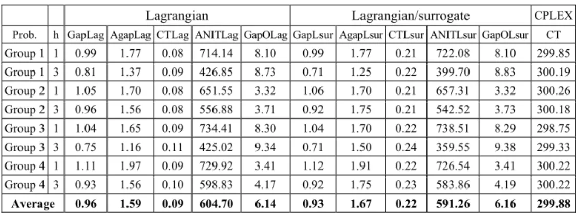
Table 1 shows the heuristic procedure results. The Lagrangian/surrogate heuristic presents solutions with average deviations smaller than the Lagrangian heuristic. Nevertheless, it cannot be said that the Lagrangian/surrogate heuristic is the best procedure for the problem since for both heuristics the stabilization and solution quality are quite similar despite the small improvement. Thus, it can be said that both approaches are competitive. In addition, Table 1 shows that the procedures have better gaps when more expensive transportation costs are considered (Groups 1 and 3).
The holding costs also affect the results found by the procedures and they are analyzed in Table 2, where group 3 is considered with various values for the holding cost.
Table 1 – Computational Results for Different parameters.
Lagrangian Lagrangian/surrogate CPLEX
Prob. h GapLag AgapLag CTLag ANITLag GapOLag GapLsur AgapLsur CTLsur ANITLsur GapOLsur CT Group 1 1 0.99 1.77 0.08 714.14 8.10 0.99 1.77 0.21 722.08 8.10 299.85
Group 1 3 0.81 1.37 0.09 426.85 8.73 0.71 1.25 0.22 399.70 8.83 300.19 Group 2 1 1.05 1.70 0.08 651.55 3.32 1.06 1.70 0.21 657.31 3.32 300.26 Group 2 3 0.96 1.56 0.08 556.88 3.71 0.92 1.75 0.21 542.52 3.73 300.18
Group 3 1 1.04 1.65 0.09 734.41 8.30 1.04 1.70 0.22 738.51 8.29 298.75 Group 3 3 0.75 1.16 0.11 425.02 9.34 0.71 1.50 0.24 359.55 9.38 299.33
Group 4 1 1.11 1.97 0.09 729.92 3.41 1.12 1.91 0.22 726.54 3.41 300.22 Group 4 3 0.93 1.56 0.10 598.83 4.17 0.92 1.75 0.23 583.86 4.19 300.22
Average 0.96 1.59 0.09 604.70 6.14 0.93 1.67 0.22 591.26 6.16 299.88
Table 2 shows that for both procedures, it can be observed that the lower the holding costs (h), the higher the average deviation, and the gaps found by the Lagrangian/surrogate heuristic (GapLsur) are better than the gaps from the Lagrangian heuristic (GapLag). Norden & Velde (2005) already highlighted this holding cost effect. When considering the holding cost equal to zero, the heuristics developed determine, on average, better quality solutions than the CPLEX. However, for elevated holding costs, CPLEX obtain better quality solutions than the heuristic proposed. It is worth mentioning that the time limit for the CPLEX to obtain a solution was set to 300 seconds for the results presented in Tables 1 and 2.
Table 2 – Computational Results for Different Holding Cost Values.
Lagrangian Lagrangian/surrogate CPLEX
Prob. h GapLag AgapLag CTLag ANITLag GapOLag GapLsur AgapLsur CTLsur ANITLsur GapOLsur CT Group 3 0 2.75 4.29 0.15 794.98 -0.51 2.70 4.17 0.30 794.74 -0.47 300.25
Group 3 0.5 1.12 1.85 0.10 779.64 7.56 1.07 1.81 0.23 777.21 7.57 300.26 Group 3 1 1.04 1.65 0.09 734.41 8.29 1.04 1.70 0.22 738.51 8.29 298.82
Group 3 2 0.86 1.50 0.09 629.73 9.07 0.86 1.53 0.23 588.45 9.08 298.73 Group 3 3 0.75 1.16 0.11 425.02 9.35 0.71 1.50 0.23 359.55 9.38 299.30 Group 3 5 0.78 1.23 0.11 289.99 9.44 0.72 1.29 0.24 225.89 9.50 300.17
Group 3 10 0.78 1.31 0.11 274.33 9.49 0.59 1.28 0.24 270.83 9.70 295.31
4.2 Results for Model (1)-(9)
The software used in these computational tests was the same used in the tests presented in Section 4.1. However, the computer used was a Pentium 4 3GHz, 1GHHz RAM.
The new data related to capacity restrictions were generated based on Trigeiro et al. (1989). The other data are similar to those described in Section 4.1. The production capacity in each period is generated depending on the production times and setup according to the following equation:
1 1
( )
1,...,
n T
i ik i
i k
t
b d q
Cap t T
T
α
= =
⎢ ⎥
+
⎢ ⎥
⎢ ⎥
= =
⎢ ⎥
⎢ ⎥
⎣ ⎦
∑∑
;
where α is a parameter for slackness capacity control and two variations are considered: α = 1 and α = 0.85 representing, respectively, the tight and normal capacities.
For all items, the time required to produce a unit of item i are given by bi = 1 and the setup times (qi) were generated randomly in the intervals [10,50] and [30,150]. Finally, there are three possibilities for delay penalties (hit−): 5, 10, or 50 times the stock cost (hit+) that was fixed in 1 or 3.
Considering the parameters defined in this section and the ones defined in Section 4.1, for each parameter combination, 100 examples are generated. A total of 9,600 examples were generated in this second step of the computational tests.
The following two tables show the results of the tests run. The problems are shown in groups with the same characteristics of Groups 1, 2, 3, and 4 described in Section 4.1. However, each group represents a 12 parameter combination (two different stock costs combined with three types of delay penalties combined with two types of different setup times). Hence, for each relative line to a group, an average of 12 combinations of these groups is presented (100 examples for each combination are generated).
For the procedures based on the Lagrangian and Lagrangian/surrogate relaxation a maximum number of 800 iterations was considered. For Lagrangian/surrogate, the initial Lagrangian multiplier µ=1 is considered and for each subgradient iteration, three iterations are applied in one-dimension searched.
Each table shows the resolution time (CPLEX was limited to 180 s in these tests), the best value obtained by CPLEX 10.0 optimization package in the time limit, the average number of iterations that the heuristics need to obtain the best solution, and the distance obtained by the heuristics in relation to the optimization.
Tables 3 and 4 show that both heuristics were again quite similar. The problem (1)-(9) can be considered more complicated due to capacity constraints and backlogging, the computational time and gap increased. A new column was included to compare the Standard Deviation (SD) of the computational time and both heuristics showed to be stable.
Table 3 – Results – Problems with tight capacity (α = 1).
Lagrangian Lagrangian/surrogate
Prob. GapLag AgapLag CTLag SD ANITLag GapOLag GapLsur AgapLsur CTLsur SD ANITLsur GapOLsur Group 1 30.63 44.83 16.89 1.81 173.84 29.77 28.69 47.95 17.50 2.08 165.36 28.44
Group 2 25.82 35.13 14.21 1.80 275.82 25.25 24.87 36.60 14.82 1.75 267.47 24.87 Group 3 31.23 48.33 16.31 1.34 177.36 30.22 29.47 52.48 16.78 1.34 148.82 29.07
Group 4 26.48 37.91 14.27 1.79 274.11 25.82 25.50 40.11 14.88 1.79 268.88 25.44 Average 28.54 41.55 15.42 1.69 225.28 27.77 27.13 44.28 16.00 1.74 212.63 26.95
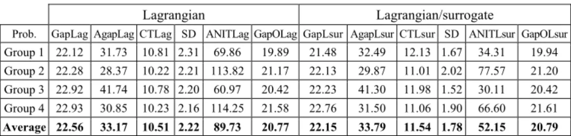
Considering the normal capacity (Table 4), it can be seen that the heuristics need less iterations to obtain the upper bound and it obtains a better upper bound. The results for the other data variations follow the same pattern of the results of the tight capacity problems.
Table 4 – Results – Problems with normal capacity (α = 0, 85).
Lagrangian Lagrangian/surrogate
Prob. GapLag AgapLag CTLag SD ANITLag GapOLag GapLsur AgapLsur CTLsur SD ANITLsur GapOLsur Group 1 22.12 31.73 10.81 2.31 69.86 19.89 21.48 32.49 12.13 1.67 34.31 19.94 Group 2 22.28 28.37 10.22 2.21 113.82 21.17 22.13 29.87 11.01 2.02 77.57 21.20
Group 3 22.92 41.74 10.78 2.20 60.97 20.42 22.23 41.30 11.98 1.52 30.11 20.42 Group 4 22.93 30.85 10.23 2.16 114.25 21.58 22.76 31.50 11.06 1.90 66.60 21.61
Average 22.56 33.17 10.51 2.22 89.73 20.77 22.15 33.79 11.54 1.78 52.15 20.79
As seen in Section 4.1 to the problem proposed by Norden & Velde (2005), the heuristics are competitive and the heuristic Lagrangian/surrogate produce gaps lower than the Lagrangian. However, we can not say that the Lagrangian/surrogate procedure is the best procedure for the problem (1)-(9), i.e., the analysis remains valid to the procedures outlined in Section 4.1.
5. Conclusions
The aim of this study was to evaluate the efficiency of the Lagrangian/surrogate approach for the integrated lot-sizing and distribution problem. The problem studied involves production and transportation planning of various items in a planning horizon of T periods. The objective is to minimize setup, production, inventory and transportation costs. Transporting items involves a contract established for the whole planning horizon and it has a fixed cost, a reduced cost for a fixed number of contracted containers, and the possibility of contracting additional containers at an elevated cost. The number of contracted containers is estimated based on the planning horizon demand forecast.
constraints, the results of the Lagrangian/surrogate heuristic are better than the Lagrangian heuristic results. It can be concluded that the approach proposed is competitive, which stimulates the study of its application in other lot-sizing and distribution problems.
Acknowledgements
The authors would like to thank the anonymous referees for their useful comments and suggestions. This research was partially funded by the Fundação de Amparo a Pesquisa do Estado de São Paulo (FAPESP), Conselho Nacional de Desenvolvimento Científico e Tecnológico (CNPq) and Coordenação de Aperfeiçoamento de Pessoal de Nível Superior (CAPES).
References
(1) Araujo, S.A. & Arenales, M.N. (2000). Problema de Dimensionamento de Lotes Monoestágio com Restrição de Capacidade: modelagem, método de resolução e resultados computacionais. Pesquisa Operacional, 20, 2, 287-306.
(2) Baumol, W.J. & Vinod, H.D. (1970). An inventory theoretic model of freight transport demand. Management Science, 16, 413-421.
(3) Bertazzi, L. & Speranza, M.G. (1999). Models and Algorithms for the Minimization of Inventory and Transportation Costs: A Survey. In: New Trends in Distribution Logistics (edited by M.G. Speranza and P. Staehly), Lecture Notes in Economics and Mathematical Systems, Vol. 480, pp. 137-157, Springer-Verlag, Berlin Heidelberg.
(4) Brahimi, N.; Dauzere-Peres, S.; Najid, N.M. & Nordi, A. (2006), Single Item Lot Sizing Problems. European Journal of Operational Research, 168, 1-16.
(5) Diaby, M.; Bahl H.; Karwan, M.H. & Ziont, S. (1992). Capacitated Lot-Sizing and Scheduling by Lagrangean Relaxation. European Journal of Operational Research, 59, 444-458.
(6) Erenguç, S.S.; Simpson, N.C. & Vakharia, A.J. (1999). Integrated production/ distribution planning in supply chains? An invited review. European Journal of Operational Research, 115, 219-236.
(7) Fisher, M.L. (1981). The Lagrangian relaxation method for solving integer programming problems. Management Science, 27, 1-18.
(8) Geoffrion, A.M. (1974). Lagrangian relaxation in integer programming. Mathematical ProgrammingStudy, 2, 82-114.
(9) Glover, F. (1965). A multiphase dual algorithm for the zero-one integer programming problem. Operations Research, 13, 879-919.
(10) Glover, F. (1968). Surrogate Constraints. Operations Research, 16(4), 741-749.
(11) Glover, F. (1975). Surrogate Constraints Duality in Mathematical Programming.
Operations Research, 23, 434-451.
(12) Greenberg, H.J. & Pierskalla, W.P. (1970). Surrogate Mathematical Programming.
(13) Greenberg, H.J. & Pierskalla, W.P. (1973). Quasi-conjugate Functions and Surrogate Duality. Cahiers Centre Études de Rech. Oper., 15, 437-448.
(14) Held, M.; Wolfe, P. & Croweder, H. (1974). Validation of Subgradient Optimization.
Mathematical Programming, 6, 62-68.
(15) Held, M. & Karp, R.M. (1971). The traveling salesman problem and minimum spanning tress: part II. Mathematical Programming, 1, 6-25.
(16) Karimi, B.; Ghomi, S.M.T.F. & Wilson, J.M. (2003). The capacitated lot sizing problem: a review of models and algorithms. Omega, 31, 365-378.
(17) Karwan, M.L. & Rardin, R.L. (1979). Some Relationships Between Lagrangean and Surrogate Duality in Integer Programming. Mathematical Programming, 17, 320-334. (18) Lee, C.Y. (1989). A solution to the multiple set-up problem with dynamic demand.
IIE Transactions, 21, 266-270.
(19) Lee, W.-S.; Han, J.H. & Cho, S.J. (2005). A heuristic for a multi-product dynamic lot-sizing and shipping problem. Int. J. Production Economics, 98, 204-214.
(20) Lorena, L.A.N. & Pereira, M.A. (2002). A lagrangean/surrogate heuristic for the maximal covering problem using Hillsman’s edition. International Journalof Industrial Engineering, 9(1), 57-67.
(21) Lozano, S.; Larraneta, J. & Oliveira, L. (1991). Primal Dual Approach to the Single Level Capacitated Lot-Sizing Problem. European Journal of Operational Research, 51, 354-366.
(22) Narciso, M.G. (1998). A relaxação Lagrangeana/Surrogate e algumas aplicações em otimização combinatória. Tese de Doutorado em Computação Aplicada, INPE, São José dos Campos.
(23) Narciso, M.G. & Lorena, L.A.N. (1999). Lagrangean/Surrogate relaxation for generalized assignment problem. European Journal of Operational Research, 114, 165-177. (24) Norden, L. van & Velde, S. van de (2005). Multi-product lot-sizing with a transportation
capacity reservation contract. European Journal of Operational Research, 165, 127-138.
(25) Oliveira, L.K. & Morabito, R. (2006). Métodos Exatos Baseados em Relaxações Lagrangiana e Surrogate para o Problema de Carregamento de Paletes do Produtor.
Pesquisa Operacional, 26, 403-432.
(26) Rizk, N. & Martel, A. (2001). Supply chain flow planning methods: a review of the lot-sizing literature. Working Paper DT-2001-AM-1, Université Laval, QC, Canada.
(27) Senne, E.L.F. & Lorena, L.A.N. (2000). Lagrangean/Surrogate Heuristics for p-Median Problems. In: Computing Tools for Modeling, Optimization and Simulation: Interfaces in Computer Science and Operations Research [edited by M. Laguna and J.L. Gonzalez-Velarde], Kluwer Academic Publishers, 115-130.
(29) Trigeiro, W.W.; Thomas, L.J. & Mcclain, J.O. (1989). Capacitated Lot Sizing With Setup Times. Management Science, 35(3), 353-366.
(30) Vroblefski, M.; Ramesh, R. & Zionts, S. (2000). Efficient lot-sizing under a differential transportation cost structure for serially distributed ware-houses. European Journal of Operational Research, 127, 574-593.