Volume 2010, Article ID 378203,25pages doi:10.1155/2010/378203
Review Article
Testing Gaussianity, Homogeneity, and Isotropy with
the Cosmic Microwave Background
L. Raul Abramo
1and Thiago S. Pereira
21Instituto de F´ısica, Universidade de S˜ao Paulo, CP 66318, CEP 05315-970 S˜ao Paulo, Brazil
2Instituto de F´ısica Te´orica, Universidade Estadual Paulista, CP 70532-2, CEP 01156-970 S˜ao Paulo, Brazil
Correspondence should be addressed to L. Raul Abramo,[email protected]
Received 3 February 2010; Accepted 12 May 2010
Academic Editor: Dragan Huterer
Copyright © 2010 L. R. Abramo and T. S. Pereira. This is an open access article distributed under the Creative Commons Attribution License, which permits unrestricted use, distribution, and reproduction in any medium, provided the original work is properly cited.
We review the basic hypotheses which motivate the statistical framework used to analyze the cosmic microwave background, and how that framework can be enlarged as we relax those hypotheses. In particular, we try to separate as much as possible the questions of gaussianity, homogeneity, and isotropy from each other. We focus both on isotropic estimators of nongaussianity as well as statistically anisotropic estimators of gaussianity, giving particular emphasis on their signatures and the enhanced “cosmic variances” that become increasingly important as our putative Universe becomes less symmetric. After reviewing the formalism behind some simple model-independent tests, we discuss how these tests can be applied to CMB data when searching for large-scale “anomalies”.
1. Introduction
According to our current understanding of the Universe, the morphology of the cosmic microwave background (CMB) temperature field, as well as all cosmological structures that are now visible, like galaxies, clusters of galaxies, and the whole web of large-scale structure, are probably the
descen-dants of quantum process that took place some 10−35seconds
after the Big Bang. In the standard lore, the machinery responsible for these processes is termed cosmic inflation and, in general terms, what it means is that microscopic quantum fluctuations pervading the primordial Universe are stretched to what correspond, today, to cosmological scales (see [1–3] for comprehensive introductions to inflation.) These primordial perturbations serve as initial conditions for the process of structure formation, which enhance these initial perturbations through gravitational instability. The subsequent (classical) evolution of these instabilities preserves the main statistical features of these fluctuations that were inherited from their inflationary origin–provided, of course, that we restrain ourselves to linear perturbation theory.
However, given that matter has a natural tendency to cluster, and this inevitably leads to nonlinearities (not to mention the sorts of complications that come with baryonic physics), the structures which are visible today are far from ideal probes of those statistical properties. CMB photons, on the other hand, to an excellent approximation experience
free streaming since the time of decoupling (z≈1100) and
are therefore exempt from these non-linearities (except, of course, for secondary anisotropies such as the Rees-Sciama
effect or the Sunyaev-Zel’dovich effect), which implies that
they constitute an ideal window to the physics of the early Universe—see, for example, [4–6]. In fact, we can determine the primary CMB anisotropies as well as most of the secondary anisotropies on large scales, such as the
Integrated Sachs-Wolfe effect, completely in terms of the
initial conditions by means of a linear kernelas follows:
Θ(n)≡∆T
n;η0
Tη0 =
d3x′ η0
0 dη ′
i
Ki−→x′,η′;nSi−→x′
,η′,
where η′ is conformal time, and Si denote the initial
conditions of all matter and metric fields (as well as their time derivatives, if the initial conditions are nonadiabatic).
Here Ki is a linear kernel, or a retarded Green’s function,
that propagates the radiation field to the time and place of its detection, here on Earth. Since that kernel is insensitive to the statistical nature of the initial conditions (which can be thought of as constants which multiply the source terms), those properties are precisely transferred to the CMB
temperature fieldΘ.
The statistical properties of the primordial fluctuations are, to lowest order in perturbation theory, quite simple; because the quantum fluctuations that get stretched and enhanced by inflation are basically harmonic oscillators in their ground state, the distribution of those fluctuations is Gaussian, with each mode an independent random variable. The Fourier modes of these fluctuations are characterized by random phases (corresponding to the random initial values of the oscillators), with zero mean, and variances which are given simply by the field mass and the mode’s
wavenumber k = 2π/λ. The presence of higher-order
interactions (which exist even for free fields, because of gravity) changes this simple picture, introducing higher-order correlations which destroy gaussianity—even in the simplest scenario of inflation [7–9]. However, since these interactions are typically suppressed by powers of the
factor GH2 ≃ 10−12, where G is Newton’s constant
and H the Hubble parameter during inflation, the
cor-rections are small—but, at least in principle, detectable [10–12].
Since these statistical properties are a generic prediction of (essentially) all inflationary models, they can also be inferred from two ingredients that are usually assumed as a first approximation to our Universe. First, since inflation was designed to stretch our Universe until it became spatially homogeneous and isotropic, it is reasonable to expect that all statistical momenta of the CMB should be spatially homogeneous and rotationally invariant, regardless of their general form. Second, in linear perturbation theory [13] where we have a large number of cosmological fluctuations
evolving independently, we can expect, based on thecentral
limit theorem, that the Universe will obey a Gaussian distribution.
The power of this program lies, therefore, in its simplic-ity: if the Universe is indeed Gaussian, homogeneous, and statistically isotropic (SI), then essentially all the information about inflation and the linear (low redshift) evolution of the Universe is encoded in the variance, or two-point correlation function, of large-scale cosmological structures and/or the CMB. As it turns out, the five-year dataset from the Wilkinson Microwave anisotropy probe (WMAP)
strongly supports these predictions [11,14]. Moreover, the
measurements of the CMB temperature power spectrum by the WMAP team, alongside measurements of the matter
power spectrum from existing survey of galaxies [15, 16]
and data from type Ia supernovae [17–19], have shown
remarkable consistency with aconcordance model(ΛCDM),
in which the cosmos figures as a Gaussian, spatially flat, approximately homogeneous, and statistically isotropic web
of structures composed mainly of baryons, dark matter, and dark energy.
However, while the detection of a nearly scale-invariant and Gaussian spectrum is a powerful boost to the idea of inflation, just knowing the variance of the primordial
fluctuations is not sufficient to single out which particular
inflationary model was realized in our Universe. For that, we will need not only the 2-point function, but the higher momenta of the distribution as well. Therefore, in order to break this model degeneracy, we must go beyond the
framework of theΛCDM, Gaussian, spatially homogeneous,
and statistically isotropic Universe.
Reconstructing our cosmic history, however, is not the only reason to explore further the statistical properties of the CMB. The full-sky temperature maps by WMAP
[11, 20] have revealed the existence of a series of
large-angle anomalies—which, incidentally, were (on hindsight) already visible in the lower-resolution COBE data [21]. These anomalies suggest that at least one of our cherished hypotheses underlying the standard cosmological model might be wrong—even as a first-order approximation. Perhaps the most intriguing anomalies (described in more detail in other review papers in this volume) are the low value of the quadrupole and its alignment of the quadrupole
(ℓ = 2) with the octupole (ℓ = 3) [22–27], the sphericity
[26] (or lack of planarity [28]), of the multipole ℓ = 5,
and the north-south asymmetry [29–33]. In the framework of the standard cosmological model, these are very unlikely statistical events, and yet the evidence that they exist in the real data (and are not artifacts of poorly subtracted extended foregrounds—e.g., [34]) is strong.
Concerning theoretical explanations, even though we
have by now an arsenal of ad hocmodels designed to account
for the existence of these anomalies, none has yet quite succeeded in explaining their origin. Nevertheless, they all share the point of view that the detected anomalies might be related to a deviation of gaussianity and/or statistical isotropy.
In this paper, we will describe, first, how to character-ize, from the point of view of the underlying spacetime symmetries, both non-gaussianity and statistical anisotropy. We will adopt two guiding principles. The first is that
gaussianity and SI, being completely different properties of
a random variable, should be treated separately, whenever possible or practical. Second, since there is only one type of gaussianity and SI but virtually infinite ways away from them, it is important to try to measure these deviations without a particular model or anomaly in mind–although we may eventually appeal to particular models as illustrations or as a means of comparison. This approach is not new and, although not usually mentioned explicitly, it has been
adopted in a number of recent papers [35,36].
One of the main motivations for this model-independent
approach is the difficult issue of aprioristicstatistics; one can
only test the random nature of a process if it can be repeated a very large (formally, infinite) number of times. Since the CMB only changes on a timescale of tens of millions of years,
waiting for our surface of last scattering to probe a different
we are stuck with one dataset (a sequence of apparently random numbers), which we can subject to any number of tests. Clearly, by sheer chance, about 30% of the tests will give a positive detection with 70% confidence level (CL), 10% will give a positive detection with 90% CL, and so on. With enough time, anyone can come up with detections of arbitrarily high significance—and ingenuity will surely accelerate this process. Hence, it would be useful to have a few guiding principles to inform and motivate our statistical tests, so that we do not end up shooting blindly at a finite number of fish in a small wheelbarrow.
This paper is divided into two parts. We start Part I by reviewing the basic statistical framework behind linear perturbation theory (Section 2). This serves as a
motivation for Section 3, where we discuss the formal
aspects of non-Gaussian and statistically isotropic models (Section 2.1), as well as Gaussian models of statistical anisotropy (Section 2.2). Part II is devoted to a discussion on model-independent cosmological tests of non-gaussianity and statistical anisotropy and their application to CMB data. We focus on two particular tests, namely, the multipole vectors statistics (Section 3) and functional modifications of the two-point correlation function (Section 4). After discussing how such tests are usually carried out when searching for anomalies in CMB data (Section 6.1), we present a new formalism which generalizes the standard procedure by including the ergodicity of cosmological data as a possible source of errors (Section 6.2). This formalism
is illustrated inSection 7, where we carry a search of
planar-type deviations of isotropy in CMB data. We then conclude
inSection 8.
Part I: The Linearized Universe
2. General Structure
We start by defining the temperature fluctuation field. Since the background radiation is known to have an average temperature of 2.725 K, we are interested only in deviations
from this value at a given directionnin the CMB sky. So let
us consider the dimensionless function onS2as follows:
Θ(n)≡T(n)−T0
T0
, (2)
where T0 = 2.725 K is the blackbody temperature of the
mean photon energy distribution—which, if homogeneity holds, is also equal to the ensemble average of the temper-ature.
In full generality, the fluctuation field is not only a
function of the position vector −→n, but also of the time in
which our measurements are taken. In practice, the time and displacement of measurements vary so slowly that we can ignore these dependences altogether. Therefore, we can equally well consider this function as one defined only on the
unit radius sphereS2, for which the following decomposition
holds:
Θ(n)=
ℓ,m
aℓmYℓm(n). (3)
Since the spherical harmonics Yℓm(n) obey the symmetry
Y∗
ℓm(n)=(−1)mYℓ,−m(n), the fact that the temperature field
is a real function implies the identity a∗
ℓm = (−1)maℓ,−m.
This means that each temperature multipoleℓis completely
characterized by 2ℓ+ 1 real degrees of freedom.
2.1. From Inhomogeneities to Anisotropies: Linear Theory.
The ultimate source of anisotropies in the Universe is the inhomogeneities in the baryon-photon fluid, as well as their associated spacetime metric fluctuations. If the photons were in perfect equilibrium with the baryons up to a sharply defined moment in time (the so-called instant recombination approximation), their distribution would have only one parameter (the equilibrium temperature at
each point), so that photons flying off in any direction
would have exactly the same energies. In that case, the
photons we see today coming from a line-of-sightnwould
reflect simply the density and gravitational potentials (the
“sources”) at the positionRn, whereRis the radius to that
(instantaneous) last scattering surface. Evidently, multiple scatterings at the epoch of recombination, combined with the fact that anisotropies themselves act as sources for more anisotropies, complicate this picture, and in general the relationship of the sources with the anisotropies must be calculated from either a set of Einstein-Boltzmann equations or, equivalently, from the line-of-sight integral equations coupled with the Einstein, continuity, and Euler equations [6].
Assuming for simplicity that recombination was
instan-taneous, at a time ηR, the linear kernels of (1) reduce to
Ki(−→x′,η′;n) →βiδ(η′−ηR)δ(−→x′−nR ), whereR=η
0−ηR
andβiare constant coefficients. The photon distribution that
we measure on Earth would therefore be given by
Θ(n)≈
i
βiSi−→x′
=nR ,η′=ηR.
(4)
We can also express this result in terms of the Fourier spectrum of the sources as follows:
Θ(n)≈
i βi
d3k
(2π)3e
i−→k·nRSi−→k,ηR.
(5)
Now we can use what is usually referred to as “Rayleigh’s expansion” (though Watson, in his classic book on Bessel functions, attributes this to Bauer, J. f. Math. LVI, 1859) as follows:
ei−→k·−→x
=4π
ℓm
iℓjℓ(kx)Y∗
ℓm
kYℓm(x), (6)
where jℓ(z) are the spherical Bessel functions. Substituting
(6) into (5) we obtain that
aℓm=
d2n Y ∗
ℓm(n)Θ(n)
≈
d3k
(2π)3Θ
−→
k×4πiℓjℓ(kR)Y∗
ℓm
k,
(7)
where we have loosely collected the sources into the term
simple relation between the Fourier modes and the spherical
harmonic modes. Therefore, up to coefficients which are
known given some background cosmology, the statistical
properties of the harmonic coefficients aℓm are inherited
from those of the Fourier modes Θ(−→k) of the underlying
matter and metric fields. Notice that the properties of the
aℓms under rotations, on the other hand, have nothing to do
with the statistical properties of the fluctuations; they come
directly from the spherical harmonic functionsYℓm.
2.2. Statistics in Fourier Space. The characterization of the statistics of random variables is most commonly expressed in terms of the correlation functions. The two-point correlation function is the ensemble expectation value,
C
−→
k,−→k′≡Θ−→kΘ
−→
k′. (8)
In the absence of any symmetries, this would be a generic
function of the arguments −→k and −→k′, with only two
constraints: first, becauseΘ(−→x) is a real function,Θ∗(−→k)=
Θ(−−→k), hence, in our definitionC∗(−→k,k→−′)=C(−→−k,−−→k′);
second, due to the associative nature of the expectation value,
C(−→k,−→k′) = C(−→k′,−→k). It is obvious how to generalize this
definition to 3, 4, or an arbitrary number of fields at different
− →
ks (or “points”).
Let us first discuss the issue of gaussianity. If we say
that the variables Θ(−→k) are Gaussian random numbers,
then all the information that characterizes their distribution
is contained in their two-point function C(−→k,−→k′). The
probability distribution function (pdf) is then formally given by
P
Θ−→k,Θ
−→
k′∼exp
⎡ ⎢
⎣−
Θ−→kΘ−→k′
2C−→k,−→k′
⎤ ⎥
⎦. (9)
In this case, all higher-order correlation functions are either zero (for odd numbers of points) or they are simply connected to the two-point function by means of Wick’s Theorem as follows:
Θ−→k1Θ−→k2· · ·Θ−→k2N
G
=
i,j N
α=1
Biα,j
Θ−→kiΘ−→kj,
(10)
where the sum runs over all permutations of the pairs of wave
vectors andBi,jare weights.
Second, let us consider the issue of homogeneity. A field is homogeneous if its expectation values (or averages) do not dependent on the spatial points where they are evaluated. In
terms of theN-point functions in real space, we should have
the following
Θ−→
x1Θ−→x2· · ·Θ−→xN
Homog.
−−−−→CN−→x1− −→x2,. . .,−→xN−1− −→xN.
(11)
Writing this expression in terms of the Fourier modes, we get the following
Θ−→
x1Θ−→x2· · ·Θ−→xN
= d3k
1d3k1· · ·d3kN
(2π)3N e
−i−→k1·−→x1e−i−→k2·−→x2· · ·e−i−→kN·−→xN
×Θ−→k1Θ→−k2· · ·Θ−→kN.
(12)
Homogeneity demands that the expression in (12) is a
function of the distances between spatial points only, not
of the points themselves. Hence, the expectation value in Fourier space on the right-hand side of this expression must
be proportional toδ(−→k1+−→k2+· · ·+−→kN).In other words, the
hypothesis of homogeneity constrains theN-point function
in Fourier space to be of the following form:
Θ−→k1Θ−→k2· · ·Θ−→kN
H
=(2π)3N−→k1,−→k2,. . .,−→kN
×δ−→k1+→−k2+· · ·+−→kN
.
(13)
Notice that the “(N −1)-spectrum” in Fourier space, N,
can still be a function of the directions of the wavenumbers
− →
ki (it will be, in fact, a function of N −1 such vectors,
due to the global momentum conservation expressed by the
δ-function.) Models which realize the general idea of (13)
correspond to homogeneous but anisotropic universes [37– 40].
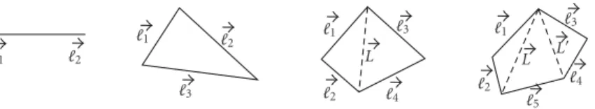
There is a useful diagrammatic illustration for the N
-point functions in Fourier space that enforce homogeneity.
Notice that we could use theδ-function in (13) to integrate
out any one of the momenta −→ki in (12). Let us instead
rewrite theδ-functions in terms of triangles, so for the
4-point function we have
δ−→k1+−→k2+−→k3+−→k4
=
d3qδ−→k1+−→k2− −→q
δ−→k3+−→k4+−→q
, (14)
whereas for the 5-point function we have
δ−→k1+−→k2+→−k3+−→k4+−→k5
=
d3qd3q′δ−→k1+−→k2− −→q
δ−→q +−→k3− −→q′
×δ−→q′+−→k4+−→k5
,
(15)
and so on, so that theN-pointδ-function is reduced toN−2
triangles withN−3 “internal momenta” (the idea is nicely
illustrated inFigure 1.) Substituting the expression for theN
momenta but the first (−→k1) and last (−→kN), the result is as
follows
Θ−→
x1Θ−→x2· · ·Θ−→xN
= 1
(2π)3N
d3k
1d3q1· · ·d3qN−3d3kN
×ei−→k1·(−→x1−−→x2)ei−→q1·(−→x2−−→x3)
· · ·ei−→qN−3·(−→xN−2−−→xN−1)
×ei−→kN·(−→xN−1−−→xN)Θ−→k
1
Θ−→q
1−
− →
k1
· · ·Θ−→kN. (16)
This expression shows explicitly that the real-spaceN-point
function above does not depend on any particular spatial point, only on the intervals between points.
Finally, what are the constraints imposed on the N
-point functions that come from isotropy alone? Clearly, no
dependence on the directionsdefined by the points,−→xi− −→xj,
can arise in the final expression for the N-point functions
in real space, so from (12) we see that theN-point function
in Fourier space should depend only on the moduli of
the wavenumbers—up to some momentum-conservationδ
-functions, which naturally carry vector degrees of freedom. In this paper, we will mostly be concerned with tests of isotropy given homogeneity (but not necessarily
Gaussian-ity), so in our case we will usually assume that theN-point
function in Fourier space assumes the form given in (13).
2.3. Statistics in Harmonic Space. In the previous Section, we characterized the statistics of our field in Fourier space, which in most cases is most easily related to fundamental models such as inflation. Now we will change to harmonic representation, because that is what is most directly related to
the observations of the CMB,Θ(n), which are taken over the
unit sphereS2. We will discuss mostly the two-point function
here, and we defer a fuller discussion ofN-point functions in
harmonic space toSection 3.
From (7), we can start by taking the two-point function in harmonic space, and computing it in terms of the two-point function in Fourier space as follows
aℓma∗
ℓ′m′
=
d3kd3k′
(2π)6 (4π)
2
iℓ(−i)ℓ′jℓ(kR)jℓ′(k′R)Yℓm
k
×Y∗
ℓ′m′
k′Θ−→kΘ∗−→k′.
(17)
Under the hypothesis of homogeneity, this expression sim-plifies considerably, leading to
aℓma∗
ℓ′m′
H
=
d3k2 πi
ℓ(
−i)ℓ′jℓ(kR)jℓ′(kR)YℓmkYℓ∗′m′
k×N2
−→
k.
(18)
If, in addition to homogeneity, we also assume isotropy,
then N2 → P(k), and the integration over angles factors
out, leading to the orthogonality condition for spherical harmonics as follows
d2k YℓmkYℓ∗′m′
k=δℓℓ′δmm′, (19)
and as a result the covariance of theaℓms becomes diagonal
as follows
aℓma∗
ℓ′m′
H,I=δℓℓ′δmm′
dk k j
2
ℓ(kR)
2
πk
3P(k)
=4π δℓℓ′δmm′
dlogk jℓ2(kR)∆2T(k)
≡Cℓδℓℓ′δmm′,
(20)
where we have defined the usual temperature power spectrum
∆T(k) = k3P(k)/2π2 in the middle line, and the angular
power spectrumCℓ in the last line of (20). As a pedagogical
note, let us recall that the power spectrum basically expresses how much power the two-point correlation function has per
unit logkas follows:
Θ−→xΘ−→x′
H,I=
dlog ksin
k−→x − −→x′
k−→x − −→x′ ∆
2
T(k).
(21)
In an analogous manner to what was done above, we can
also construct theangulartwo-point correlation function in
harmonic space as follows:
Θ
(n)Θ(n′)=
ℓm
ℓ′m′
aℓma∗
ℓ′m′Yℓm(n)Yℓm∗(n′). (22)
The hypothesis of homogeneity by itself does not lead to significant simplifications, but isotropy leads to a very intuitive expression for the angular two-point function as follows:
Θ
(n)Θ(n′)H,I=
ℓm
ℓ′m′
Cℓδℓℓ′δmm′Yℓm(n)Yℓm∗(n′)
=
ℓ
Cℓ2ℓ+ 1
4π Pℓ(n·n
′).
(23)
Clearly, not only is this expression the analogous in S2 of
(21), but in fact the Fourier power spectrum∆2
T(k) and the
angular power spectrumCℓare defined in terms of each other
as indicated in (23) as follows:
Cℓ=4π
dlogk j2
ℓ(kR)∆2T(k). (24)
Now, using the facts that the spherical Bessel function of
orderℓpeaks when its argument is approximately given by
ℓ, and that dlogz jℓ2(z) = 1/(2ℓ(ℓ+ 1)), we obtain the
following (this is one type of what has become known in the
literature as Limber’s approximations)
Cℓ≈ 2π
ℓ(ℓ+ 1)∆
2
T
k= ℓ
R
k1 k2 k1
k3
k2 k1 k3
q
k4 k2
k1 k3
q q′
k2 k5
k4
Figure1: Diagrammatic representation of the 2, 3, 4, and 5-point correlation functions in Fourier space. The dashed lines represent internal
momenta.
Incidentally, from this expression it is clear why it is customary to define
Cℓ≡ℓ
(ℓ+ 1)
2π Cℓ≈∆
2
T
k=Rℓ
. (26)
Using (12), we can easily generalize the results of this
subsection toN-point functions inS2and in harmonic space,
however, the assumption of isotropy alone does very little to simplify our life. The hypothesis of homogeneity, on the
other hand, greatly simplifies the angularN-point functions,
and most of the work in statistical anisotropy of the CMB that goes beyond the two-point function assumes that homogeneity holds. Notice that the issue of gaussianity is, as always, confined to the question of whether or not the two-point function holds all information about the distribution of the relevant variables and is therefore completely separated from questions about homogeneity and/or isotropy.
Also notice that the separable nature of the definition (22) implies here as well, like in Fourier space, a reciprocity relation for the correlation function
C(n1,n2)=C(n2,n1). (27)
This symmetry must hold regardless of underlying models and is important in order to analyze the symmetries of the correlation function, as we will see later.
Before we move on, it is perhaps important to mention that the decomposition (22) is not unique. In fact, instead of
the angular momenta of the parts, (ℓ1,m1;ℓ2,m2), we could
equally well have used the basis of total angular momentum
(L,M;ℓ1,ℓ2) and decomposed that expression as
C(n1,n2)=
L,M
ℓ1,ℓ2
ALMℓ1ℓ2YLMℓ1ℓ2(n1,n2), (28)
whereYLMℓ1ℓ2 are known as the bipolar spherical harmonics,
defined by [41]
YLMℓ1ℓ2(n1,n2)=Yℓ1(n1)⊗Yℓ2(n2)
LM, (29)
whereLandM=m1+m2are the eigenvalues of the total and
azimuthal angular momentum operators, respectively. This decomposition is completely equivalent to (22), and we can exchange from one decomposition to another by using the relation
ALMℓ1ℓ2=
m1m2
aℓ1m1aℓ2m2
(−1)M+ℓ1−ℓ2√2
L+ 1 ℓ1 ℓ2 L
m1 m2 −M
!
,
(30)
where the 3 ×2 matrices above are the well-known 3-j
coefficients. At this point, it is only a matter of mathematical
convenience whether we choose to decompose the correla-tion funccorrela-tion as in (22) or as in (28). Although the bipolar harmonics behave similarly to the usual spherical harmonics in many aspects, the modulations of the correlation function as described in this basis have a peculiar interpretation. We will not go further into detail about this decomposition here, as it is discussed at length in another review article in this volume.
2.4. Estimators and Cosmic Variance. Returning to the covariance matrix (20), we see that, if we assume gaussianity
of the aℓms, then the angular power spectrum suffices to
describe statistically how much the temperature fluctuates in any given angular scale; all we have to do is to calculate the average (20). This can be a problem, though, since we have only one Universe to measure, and therefore only one
set of aℓms. In other words, the average in (20) is poorly
determined.
At this point, the hypothesis that our Universe is spatially homogeneous and isotropic at cosmological scales comes not only as simplifying assumption about the spacetime symmetries, but also as a remedy to this unavoidable smallness of the working cosmologist’s sample space. If
isotropy holds, different cosmological scales are statistically
independent, which means that we can take advantage of the ergodic hypothesis and trade averaging over an ensemble
for averaging over space. In other words, for a given ℓ
we can consider each of the 2ℓ + 1 real numbers in aℓm
as statistically independent Gaussian random variables, and
define astatistical estimatorfor their variances as the average
Cℓ≡ 2ℓ1+ 1
ℓ
m=−ℓ
|aℓm|2. (31)
The smaller the angular scales (ℓ bigger), the larger the
number of independent patches that the CMB sky can be divided into. Therefore, in this limit we should have
lim
ℓ→ ∞Cℓ =Cℓ. (32)
On the other hand, for large angular scales (smallℓ’s), the
number of independent patches of our Universe becomes
smaller, and (31) becomes a weak estimation of theCℓs. This
means that any statistical analysis of the Universe on large
scales will be plagued by this intrinsiccosmic sample variance.
Finally, it is important to keep in mind the clear
distinction between the angular power spectrumCℓ and its
estimator (31). The former is a theoretical variable which can be calculated from first principles, as we have shown in Section 2.1. The latter, being a function of the data, is itself
a random variable. In fact, if theaℓms are Gaussian, then we
can rewrite expression (31) as
(2ℓ+ 1)
Cℓ Cℓ =Xℓ, Xℓ=
ℓ
m=−ℓ
|aℓm|2
Cℓ , (33)
whereXℓis a chi-square random variable with 2ℓ+ 1 degrees
of freedom. According to the central limit theorem, when
ℓ → ∞, Xℓ approaches a standard normal variable (A
standard normal variable is a Gaussian variableXwith zero
mean and unit variance. Any other Gaussian variableYwith
mean µand variance σ can be obtained from X through
Y = σX + µ.) which implies that Cℓ will itself follow a
Gaussian distribution. Its mean can be easily calculated using (20) and (31) and is of course given by
Cℓ=Cℓ, (34)
which shows that theCℓs are unbiasedestimators of theCℓs.
It is also straightforward to calculate its variance (valid for
anyℓ)
Cℓ−CℓCℓ′−Cℓ′
=2ℓ2+ 1C2
ℓδℓℓ′. (35)
Because this estimator does not couple different
cosmologi-cal scosmologi-cales, it has the minimumcosmic variancewe can expect
from an estimator due to the finiteness of our sample—so
it isoptimalin that sense.Cℓ is therefore the best estimator
we can build to measure the statistical properties of the
multipolar coefficientsaℓmwhen both statistical isotropy and
gaussianity hold.
In later Sections, we will explore angular or harmonic
N-point functions for which the assumption of isotropy
does not hold. However, it is important to remember at all times that we have only one map, which means one set of
aℓms. The estimator for the angular power spectrum, Cℓ,
takes into account all theaℓms by dividing them into the
differentℓs and summing over all m ∈ (−ℓ,ℓ). Clearly, it
will inherit a sample variance for smallℓs, when theaℓms can
only be divided into a few “independent parts”. As we try to
estimate higher-order objects such as theN-point functions,
we will have to subdivide theaℓm’s into smaller and smaller
subsamples, which are not necessarily independent (in the statistical sense) of each other. So, the price to pay for aiming at higher-order statistics is a worsening of the cosmic sample variance.
2.5. Correlation and Statistical Independence. The covariance given in (20) has two distinct, important properties. First,
note that its diagonal entries, the Cℓ’s, are m-independent
coefficients; this is crucial for having statistical isotropy, as we
will show latter. Second, statistical isotropy at the Gaussian
level implies that different cosmological “scales” (understood
here as meaning the modes with total angular momentum
ℓ and azimuthal momentum m) should be statistically
independent of each other—and this is represented by the Kronecker deltas in (20).
In fact, statistical independence of cosmological scales is a particular property of Gaussian and statistically isotropic random fields and is not guaranteed to hold when gaus-sianity is relaxed. We will see in the next Section that the rotationally invariant 3-point correlation function (and in
general anyN >2 correlation function) couples to the three
scales involved. In particular, if it happens that the Gaussian contribution of the temperature field is given by (20), but at least one of its non-Gaussian moments are nonzero, then the fact that a particular correlation is zero, like for example
a2m1a∗3m2, does not imply that the scalesℓ = 2 and ℓ =
3 are (statistically) independent. This is just a restatement of the fact that, while statistical independence implies null correlation, the opposite is not necessarily true. This can be illustrated by the following example: consider a random
variableαdistributed as
P(α)= ⎧ ⎨ ⎩
1, α∈[0, 1],
0, otherwise. (36)
Let us now define two other variables x = cos(2πα) and
y=sin(2πα). From these definitions, it follows thatxandy
are statistically dependent variables, since knowledge of the
mean/variance ofxautomatically gives the mean/variance of
y. However, these variables are clearly uncorrelated
xy = 1
2π
2π
0 cosηsinη dη=0.
(37)
Although correlations are among cosmologist’s most popular tools when analyzing CMB properties, statistical indepen-dence may turn out to be an important property as well, specially at large angular scales, where cosmic variance is more of a critical issue.
3. Beyond the Standard Statistical Model
Until now we have been analyzing the properties of Gaussian and statistically isotropic random temperature fluctuations. This gives us a fairly good statistical description of the Universe in its linear regime, as confirmed by the astonishing
success of the ΛCDM model. This picture is incomplete
though, and we have good reasons to search for deviations of either gaussianity and/or statistical isotropy. For example, the observed clustering of matter in galactic environments certainly goes beyond the linear regime where the central limit theorem can be applied, therefore leading to large deviations of gaussianity in the matter power spectrum statistics. Besides, deviations of the cosmological principle may leave an imprint in the statistical moments of cosmolog-ical observables, which can be tested by searching for spatial inhomogeneities [42] or directionalities [43].
otherwise? This is in fact an ambitious endeavor, which may strongly depend on observational and theoretical hints on the type of signatures we are looking for. In the absence of extra input, it is important to classify these signatures
in a general scheme, differentiating those which are
non-Gaussian from those which are anisotropic. Furthermore, given that the signatures of non-gaussianity may in principle
be quite different from that of statistical anisotropy, such
a classification is crucial for data analysis, which requires sophisticated tools capable of separating these two issues. (Although gaussianity and homogeneity/isotropy are mathe-matically distinct properties, it is possible for a Gaussian but inhomogeneous/anisotropic model to look like an isotropic and homogeneous non-gaussian model. See, e.g., [44].)
We therefore startSection 3.1by analyzing deviations of
gaussianity when statistical isotropy holds. In Section 3.2,
we keep the hypothesis of gaussianity and analyze the consequences of breaking statistical rotational invariance.
3.1. Non-Gaussian and SI Models
3.1.1. Rotational Invariance ofN-Point Correlation Functions.
We turn now to the question of non-Gaussian but statistically isotropic probabilities distributions. We will keep working
with theN-point correlation function defined in harmonic
space,
aℓ1m1aℓ2m2. . . aℓNmN
, (38)
since knowledge of these functions enables one to fully reconstruct the CMB temperature probability distribution.
Specifically, we would like to know the form of any N
-point correlation function which is invariant under arbi-trary 3-dimensional spatial rotations. When rotated to a
new (primed) coordinate system, the N-point correlation
function transforms as
aℓ1m′1aℓ2m′2. . . aℓNm′N
=
allm
aℓ1m1aℓ2m2. . . aℓNmN
Dℓ1
m′
1m1D
ℓ2
m′
2m2· · ·D
ℓn m′NmN,
(39)
where theDℓ
mim′
i(α,β,γ)s are the coefficients of the Wigner
rotation-matrix, which depend on the three Euler-angles
α,β, andγ characterizing the rotation. Notice that in this
notation the primed (rotated) system is indicated by the
primed ms. For the 2-point correlation function, we have
already seen that the well-known expression
aℓ1m1aℓ2m2
=(−1)m2Cℓ
1δℓ1ℓ2δm1,−m2 (40)
does the job
aℓ1m′1aℓ2m′2
=Cℓ1
⎛
⎝
m1
(−1)m1
Dℓ1
m′
1m1D
ℓ1
m′
2−m1
⎞ ⎠δℓ1ℓ2
=(−1)m′2Cℓ
1δℓ1ℓ2δm′1,−m′2.
(41)
Note the importance of theangular spectrum,Cℓ, being an
m-independent function.
What about the 3-point function? In this case, the invariant combination is found to be
aℓ1m1aℓ2m2aℓ3m3
=Bℓ1ℓ2ℓ3
ℓ1 ℓ2 ℓ3
m1 m2 m3
!
(42)
which can be verified by straightforward calculations. Again, the nontrivial physical content of this statistical moment
is contained in an arbitrary but otherwise m-independent
function: thebispectrumBℓ1ℓ2ℓ3[45–47]. As we anticipated in
Section 2, rotational invariance of the 3-point correlation is not enough to guarantee statistical independence of the three cosmological scales involved in the bispectrum, although in principle a particular model could be formulated to ensure
thatBℓ1ℓ2ℓ3 ∝δℓ1ℓ2δℓ2ℓ3, at least for some subset of a general
geometric configuration of the 3-point correlation function.
These general properties hold for all the N-point
cor-relation function. For the 4-point corcor-relation function, for example, Hu [48] has found the following rotationally invariant combination
aℓ1m1. . . aℓ4m4
=
LM Qℓ1ℓ2
ℓ3ℓ4(L)(−1)
M ℓ1 ℓ2 L
m1 m2 −M
!
ℓ3 ℓ4 L
m3 m4 M
!
,
(43)
where theQℓ1ℓ2
ℓ3ℓ4(L) function is known as thetrispectrum, and
Lis an internal angular momentum needed to ensure parity
invariance. In a likewise manner, it can be verified that the following expression
aℓ1m1· · ·aℓ5m5
=
LM
L′M′
Pℓ1ℓ2
ℓ3ℓ4ℓ5(L,L
′)(−1)M+M′ ℓ1 ℓ2 L
m1 m2 −M
!
× mℓ3 ℓ4 L′
3 m4 −M′
!
ℓ5 L L′
m5 M M′
!
(44)
gives the rotationally invariant quadrispectrumPℓ1ℓ2
ℓ3ℓ4ℓ5(L,L′).
The examples above should be enough to show how the general structure of these functions emerges under SI; apart
from anm-independent function, every pair of momentaℓi
in these functions are connected by a triangle, which in turn connects itself to other triangles through internal momenta
when more than 3 scales are present. InFigure 2, we show
some diagrams representing the functions above.
Although we have always shown N-point functions
which are rotationally invariant, the procedure used for obtaining them was rather intuitive, and therefore does not
offer a recipe for constructing general invariant correlation
functions. Furthermore, it does not guarantee that this
procedure can be extended for arbitrary Ns. Here we will
present a recipe for doing that, which also guarantees the uniqueness of the solution.
The general recipe for obtaining the rotationally
ℓ1 ℓ2 ℓ1
ℓ3
ℓ2 ℓ1 ℓ3
L
ℓ4 ℓ2
ℓ1 ℓ3
L L
′
ℓ2 ℓ5
ℓ4
Figure2: Diagrammatic representation of the 2, 3, 4, and 5-point correlation functions in harmonic space. Here−→ℓ actually represents the
pair (ℓ,m).
(39) above, we start by contracting every pairs of Wigner functions, where by “contracting” we mean using the identity
Dℓ1
m′
1m1(ω)D
ℓ2
m′
2m2(ω)=
L,M,M′
ℓ1 ℓ2 L
m′
1 m′2 −M
!
ℓ1 ℓ2 L
m1 m2 −M′
!
×(2L+ 1)(−1)M+M′DLM′M(ω),
(45)
and whereω= {α,β,γ}is a shortcut notation for the three
Euler angles. Once this contraction is done, there will remain
N/2D-functions, which can again be contracted in pairs. This
procedure should be repeated until there is only one Wigner function left, in which case we will have an expression of the following form:
aℓ1m1· · ·aℓNmN
=
allm′
aℓ1m′1· · ·aℓNm′N
×geometrical factors×DLMM′(ω).
(46)
Now, we see that the only way for this combination to be
rotationally invariant is when the remainingDMML ′function
above does not depend onω, that is,DLMM′(ω)=δL0δM0δM′0.
Once this identity is applied to the geometrical factors, we
are done, and the remaining terms inside the primed m
-summation will give the rotationally invariant (N −
1)-spectrum.
As an illustration of this algorithm, let us construct the rotationally invariant spectrum and bispectrum. For the 2-point function, there is only one contraction to be done, and after we simplify the last Wigner function, we arrive at
aℓ1m1aℓ2m2
=
⎡ ⎢ ⎢
⎣
m′
1
aℓ1m′1
2
2ℓ1+ 1
⎤ ⎥ ⎥
⎦(−1)m2δℓ1ℓ2δm1,−m2, (47)
where, of course
Cℓ≡2ℓ1+ 1
m
|aℓm|2 (48)
is the well-known definition of the temperature angular spec-trum. For the 3-point function, there are two contractions, and the simplification of the last Wigner function gives
aℓ1m1aℓ2m2aℓ3m3
= ⎡
⎣
m′1,m′2,m′
3
aℓ1m′1aℓ2m′2aℓ3m′3
ℓ1 ℓ2 ℓ3
m′
1 m′2 m′3
!⎤
⎦ ℓ1 ℓ2 ℓ3
m1 m2 m3
!
.
(49)
From this expression and the ortoghonality of the 3-js symbols (see the Appendix), we can immediately identify the definition of the bispectrum as follows:
Bℓ1ℓ2ℓ3≡
m1,m2,m3
aℓ1m1aℓ2m2aℓ3m3
ℓ1 ℓ2 ℓ3
m1 m2 m3
!
. (50)
It should be mentioned that this recipe not only enables
us to establish the rotational invariance of any N-point
correlation function, but it also furnishes a straightforward
definition of unbiased estimators for theN-point functions.
All we have to do is to drop the ensemble average of
the primed aℓm’s. So, for example, for the 2- and
3-point functions above, the unbiased estimators are given, respectively, by
Cℓ= 1
2ℓ+ 1
m aℓma∗
ℓm,
Bℓ1ℓ2ℓ3=
m1,m2,m3
aℓ1m1aℓ2m2aℓ3m3
⎛
⎝ℓ1 ℓ2 ℓ3
m1 m2 m3
⎞ ⎠.
(51)
Notice that isotropy plays the same role, in S2, that
homogeneity plays inR3. What enforces homogeneity inR3
is the Fourier-spaceδ-functions, as in the discussion around
Figure 1. However, in S2, the equivalents of the Fourier
modes are the harmonic modes, for which there is only a
discrete notion of orthogonality—and no Diracδ-function.
What we found above is that the Wigner 3-j symbols play
the same role as the Fourier space δ-functions; they are
the enforcers of isotropy (rotational invariance) for theN
-point angular correlation function. Hence, the diagrammatic
representations of the constituents of theN-point functions
in Fourier (Figure 1) and in harmonic space (Figure 2) really
do convey the same physical idea—one inR3, the other inS2.
3.2. Gaussian and Statistically Anisotropic Models. In the last Section, we have developed an algorithm which enables
one to establish the rotational invariance of any N-point
correlation function. As we have shown, this is also an algorithm for building unbiased estimators of non-Gaussian correlations. In this Section, we will change the perspective and analyze the case of Gaussian but statistically anisotropic models of the Universe.
spacetime is sufficiently anisotropic at the onset of inflation [39]. Another source of anisotropy may result from our
inability to efficiently clean foreground contaminations from
temperature maps. Usually, the cleaning procedure involves the application of a mask function in order to eliminate contaminations of the galactic plane from raw data. As a consequence, this procedure may either induce, as well as hide some anomalies in CMB maps [28].
It is important to mention that these two examples can be perfectly treated as Gaussian: in the first case, the anisotropy of the spacetime can be established in the linear regime of perturbation theory and therefore will not destroy gaussianity of the quantum modes, provided that they are initially Gaussian. In the second case, the mask acts linearly over the temperature maps, therefore preserving its probability distribution [49].
3.2.1. Primordial Anisotropy. Recently, there have been many attempts to test the isotropy of the primordial Universe through the signatures of an anisotropic inflationary phase
[38–40, 50, 51]. A generic prediction of such models is
the linear coupling of the scalar, vector, and tensor modes through the spatial shear, which is in turn induced by anisotropy of the spacetime [38]. Whenever that happens, the matter power spectrum, defined in a similar way as in (13), will acquire a directionality dependence due to this type of see-saw mechanism. This dependence can be accommodated in a harmonic expansion of the form
P−→k=
ℓ,m
rℓm(k)Yℓmk, (52)
where the reality of P(−→k) requires that rℓm(k) =
(−1)mrℓ∗,−m(k). Given that temperature perturbationsΘ(−→x)
are real, their Fourier components must satisfy the relation
Θ(−→k) = Θ∗(−−→k). This property taken together with the
definition (13) implies that
P−→k=P−−→k, (53)
which in turn restricts theℓs in (52) to even values. Also, note
that by relaxing the assumption of spatial isotropy, we are only breaking a continuous spacetime symmetry, but discrete symmetries such as parity should still be present in this class of models. Indeed, by imposing invariance of the spectrum
under the transformationz → −z, we find that (−1)ℓ−m =
1. Similarly, invariance under the transformationsx → −x
andy → −yimplies the conditionsrℓm =(−1)mrℓ,−m and
rℓm=rℓ,−m, respectively. Gathering all these constraints with
the parity ofℓ, we conclude that
rℓm∈R, ℓ,m∈2N. (54)
That is, from the initial 2ℓ+1 degrees of freedom, onlyℓ/2+1
of them contribute to the anisotropic spectrum [39].
3.2.2. Signatures of Statistical Anisotropies. The selection rules (54) are the most generic predictions we can expect
from models with global break of anisotropy. We will now work out the consequences of these rules to the temperature power spectrum and check whether they can say something about the CMB large-scale anomalies.
From the expressions (17) and (52), we can immediately calculate the most general anisotropic covariance matrix [37] as follows
aℓ1m1a∗ℓ2m2
=
ℓ3,m3
Gℓ1ℓ2ℓ3
m1m2m3H
ℓ3m3
ℓ1ℓ2 , (55)
where
Gℓ1ℓ2ℓ3
m1m2m3=(−1)
m1
)
(2ℓ1+ 1)(2ℓ2+ 1)(2ℓ3+ 1)
4π
× ℓ0 0 01 ℓ2 ℓ3
!
ℓ1 ℓ2 ℓ3
−m1 m2 m3
! (56)
are the Gaunt coefficients resulting from the integral of three
spherical harmonics (see the Appendix). These coefficients
are zero unless the following conditions are met:
ℓ1+ℓ2+ℓ3∈2N,
m1+m2+m3=0,
ℓi−ℓj≤ℓk≤ℓi+ℓj, ∀i,j,k∈ {1, 2, 3}.
(57)
The remaining coefficients in (55) are given by
Hℓ3m3
ℓ1ℓ2 =4πi
ℓ1−ℓ2
∞
0 dlogkrℓ3m3(k)jℓ1(kR)jℓ2(kR) (58)
and correspond to the anisotropic generalization of temper-ature power spectrum (20).
The selection rules (57), taken together with (54), lead
to important signatures in the CMB. In particular, sinceℓ3is
even, the quantityℓ1±ℓ2must also be even, that is, multipoles
with different parity do not couple to each other in this class
of models
aℓ1m1a∗ℓ2m2
=0, ℓ1+ℓ2=odd. (59)
This result is in fact expected on theoretical grounds, because by breaking a continuous symmetry (isotropy) we cannot expect to generate a discrete signature (parity) in CMB. However, notice that the absence of correlations between, say, the quadrupole and the octupole, does not imply that there will be no alignment between them. One example of
this would be a covariance matrix of the formCℓmδℓℓ′δmm′. If
theCℓ,0happens to be zero, for example, then all multipoles
will present a preferred direction (in this case, thez-axis).
3.2.3. Isotropic Signature of Statistical Anisotropy. We have just shown that a generic consequence of an early anisotropic phase of the Universe is the generation of even-parity signatures in CMB maps. Interestingly, these signatures may be present even in the isotropic angular spectrum, since the
Cℓs acquire some additional modulations in the presence of
be constrained by measuring aneffectiveangular spectrum of the form
aℓma∗
ℓm
=Cℓ+ǫ
ℓ′>0
Gℓℓℓm,−′m,0Hℓ
′0
ℓℓ , (60)
where we have introduced a smallǫ parameter to quantify
the amount of primordial anisotropy.
In order to constrain these modulations, we have to build
a statistical estimator foraℓma∗ℓm. Since we are looking for
the diagonal entries of the matrix (55), a first guess would be
Ceff
ℓ =
1
2ℓ+ 1
ℓ
m=−ℓ aℓma∗
ℓm. (61)
To check whether this is an unbiased estimator of the effective
angular spectrum, we apply it to (55) and take its average
Ceff
ℓ
=Cℓ+ǫ
ℓ′>0,m
Gℓℓℓm,−′m,0Hℓℓℓ′0. (62)
Using the definition (56) of the Gaunt coefficients, them
-summation in the expression above becomes [41]
m
(−1)ℓ−m ℓ ℓ ℓ′
m −m 0
!
=*2ℓ+ 1δℓ′,0=0, (63)
where the last equality follows becauseℓ′>0. Consequently,
we conclude that
Ceℓff
=Cℓ=/aℓma∗
ℓm
. (64)
At first sight, this result may seem innocuous, showing only that this is not an appropriate estimator for (60). Note, however, that (61) is in fact the estimator of the angular spectrum usually applied to CMB data under the assumption of statistical isotropy. In other words, by means of the usual procedure we may be neglecting important information about statistical anisotropy. Moreover, the cosmic variance induced by the application of this estimator on anisotropic CMB maps is small, because, as it can easily be checked,
Ceℓff−Cℓ
Cℓeff′ −Cℓ′
=2ℓ2+ 1Cℓ2δℓℓ′+Oǫ2. (65)
This result shows that the construction of statistical estimators strongly depends on our prejudices about what non-gaussianity and statistical anisotropy should look like. Consequently, an estimator built to measure one particular property of the CMB may equally well hide other important signatures. One possible solution to this problem is to let the construction of our estimators be based on what the observations seem to tell us, as we will do in the next section.
Part II: Cosmological Tests
So much for mathematical formalism. We will now turn to the question of how the hypotheses of gaussianity and statistical isotropy of the Universe can be tested. Though we are primarily interested in applying these tests to CMB temperature maps, most of the tools we will be dealing with
can be applied to polarization (E- andB-mode maps) and to
catalogs of large-scale structures as well.
Testing the gaussianity and SI of our Universe is a difficult
task. Specially because, as we have seen, there is only one Gaussian and SI Universe, but infinitely many universes which are neither Gaussian nor isotropic. So what type of non-gaussianity and statistical anisotropy should we test for? In order to attack this problem, we can follow two
different routes. In the bottom-up approach, models for
the cosmic evolution are formulated in such a way as to account for some specific deviations from gaussianity and SI. These physical principles range from nontrivial cosmic topologies [52–54], primordial magnetic fields [55–59], and
local [43, 60–62] and global [38–40, 50] manifestation of
anisotropy, to nonminimal inflationary models [51,63–67].
The main advantage of the bottom-up approach is that we know exactly what feature of the CMB is being measured.
One of its drawbacks is the plethora of different models and
mechanisms that can be tested.
The second possibility is the top-down, or
model-independent approach. Here, we are not concerned with the mechanisms responsible for deviations of gaussianity or SI, but rather with the qualitative features of any such deviation. Once these features are understood, we can use them as a guide for model building. Examples here include
constructs ofa posterioristatistics [29,35,36] and functional
modifications of the two-point correlation function [28,37,
68–71].
In the next Section, we will explore two different
model-independent tests: one based on functional modifications of the two-point correlation function, and another one based on the so-called Maxwell’s multipole vectors.
4. Multipole Vectors
Multipole vectors were first introduced in cosmology by Copi et al. [23] as a new mathematical representation for the
primordial temperature field, where each of its multipolesℓ
are represented byℓunit real vectors. Later, it was realized
that this idea is in fact much older [72], being proposed
originally by J. C. Maxwell in his Treatise on Electricity and
Magnetism.
The power of this approach is that the multipole vectors can be entirely calculated in terms of a temperature map, without any reference to external reference frames. This makes them ideal tools to test the morphology of CMB maps, like the quadrupole-octupole alignment.
The purpose of the following presentation is only comprehensiveness. A mathematically rigorous introduction to the subject can be found in references [72–74], as well as other papers in this review volume.
4.1. Maxwell’s Representation of Harmonic Functions. We start our presentation of the multipole vectors by recalling some terminology. A harmonic function in three dimensions
is any (twice differentiable) functionhthat satisfies Laplace’s
equation