Heuristic Placement Routines for Two-Dimensional Bin Packing Problem

ISSN 1549-3644

© 2009 Science Publications

Corresponding Author: Lai Soon Lee, Department of Mathematics, Faculty of Science, University Putra Malaysia, 43400 UPM Serdang, Selangor, Malaysia Tel: +603 8946 8454 Fax: +603-8943 7958

Heuristic Placement Routines for Two-Dimensional Bin Packing Problem

1

L. Wong and

L.S. Lee

Department of Mathematics, Faculty of Science,

University Putra Malaysia, 43400 UPM Serdang, Selangor, Malaysia

Laboratory of Applied and Computational Statistics, Institute for Mathematical Research,

University Putra Malaysia, 43400 UPM Serdang, Selangor, Malaysia

Abstract. Problem statement: Cutting and packing (C and P) problems are optimization problems that are concerned in finding a good arrangement of multiple small items into one or more larger objects. Bin packing problem is a type of C AND P problems. Bin packing problem is an important industrial problem where the general objective is to reduce the production costs by maximizing the utilization of the larger objects and minimizing the material used. Approach: In this study, we considered both oriented and non-oriented cases of Two-Dimensional Bin Packing Problem (2DBPP) where a given set of small rectangles (items), was packed without overlaps into a minimum number of identical large rectangles (bins). We proposed heuristic placement routines called the Improved Lowest Gap Fill, LGFi and LGFiOF for solving non-oriented and oriented cases of 2DBPP respectively.

Extensive computational experiments using benchmark data sets collected from the literature were conducted to assess the effectiveness of the proposed routines. Results: The computational results were compared with some well known heuristic placement routines. The results showed that the LGFi and LGFiOF are competitive when compared with other heuristic placement routines. Conclusion: Both

LGFi and LGFiOF produced better packing quality compared to other heuristic placement routines.

Key words: Bin packing problem, heuristic placement, cutting and packing

INTRODUCTION

Generally, Cutting and Packing (C and P) Problems can be summarized as follows[10]:

“Given two sets of elements, namely, a set of large objects (input, supply) and a set of small items (output, demand) which are defined in one, two, or an even larger number of geometric dimensions. Then some or all the small items will be grouped into one or more subsets and assign each of them into one of the larger objects with the conditions all small items of the subset lie entirely within the large object and the small items are not overlapping”

The C and P problems contribute to many areas of application in business and industry such as in metal, wood, glass and textile industries, newspaper paging and cargo loading. The objective of the allocation process is to maximize the utilization of the larger objects or maximizing the number of items to be packed in the larger objects.

In this study, we consider oriented and non-oriented cases of two-dimensional rectangular single bin size bin packing problems which known as 2DRSBSBPP in Wäscher et al.[10]. According to Lodi et al.[8], the problem can be defined as follows:

“Given a set of n rectangular items j∈J = {1, 2,…, n}, each item j is defined by a height hj

and a width wj and an unlimited number of

rectangular bins, each having a height H and width W. The objective is to allocate without overlaps, all the rectangles into the minimum number of bins”

For the oriented case, the rectangles have fixed orientation while the rectangles can be rotated at 90° in non-oriented case of 2DBPP. This problem is classified as a class of NP-hard problem by[6].

arrangement of the layout which give the highest utilization of the metal. The oriented case of 2DBPP can contributes in newspaper paging process where the pieces of pages in newspaper are the bins and the news or advertisements (with fixed orientation) are the items. The purpose is to arrange the maximum numbers of news into minimum number of pages.

Most of the classical placement routines for 2DBPP work on levels heuristics where the packing is obtained by placing the rectangles in row from left to right which form levels. The first level is at the bottom edge of the bin while the subsequence levels in the bin are the horizontal line denoted by the top edge of the tallest rectangle packed on the level below. Coffman et al.[4] suggested three classical strategies for level packing which are summarized in Table 1 (note j = current rectangle).

In this study, we consider Bottom-Left Fill (BLF)[3], Lowest Gap Fill (LGF)[7], Touching Perimeter (TP)[8], Floor Ceiling (FC)[8] and Alternate Direction (AD)[8], which are some well known heuristic placement routines for solving the problem.

The BLF routine places the rectangles by searching through a list of location points in bottom left ordering sequence that indicates potential positions where the rectangle may be placed. Meanwhile, TP will first initialize L bins (where L is the lower bound) before packing the rectangle at the bin and position which give the highest score (percentage of the rectangle perimeter which touches the bin and the others rectangles that have been packed). The FC is a two-phase placement routine. In the first phase, the current rectangle will be packed on a floor, according to Best-Fit strategy or on a ceiling if the rectangle cannot be packed on the floor below. If neither floor nor ceiling at that level can fit the rectangle, a new level is initialized. In the second phase, the levels are packed into finite bins either through the Best-Fit Decreasing (BFD) algorithm or by using an exact algorithm for the one-dimensional bin packing problem. BFD algorithm is referred to the rectangles that are initially sorted in decreasing width, height or area following by the BF routine. For the AD,

Table 1: Classical strategies for levels packing Packing strategy Description

Next-Fit (NF) Rectangle j is packed left justified on a level if it fits. Otherwise, the level is closed and a new level is created to pack the rectangle left justified. First-Fit (FF) Rectangle j is packed left justified on the first

level where it fits. If there are no level can pack j, a new level is initialized as in NF.

Best-Fit (BF) Rectangle j is packed left justified on that level, among those where it fits, for which the resulting packing has the minimum remaining horizontal space. If no level can accommodate j, a new level is initialized as in NF.

the routine is started by sorting the items according to non-increasing heights and L (lower bound) bins are initialized by packing on their bottoms a subset of the rectangles, following best-fit decreasing policy. The remaining rectangles are packed into the bands according to the current direction associated with the bin. The LGF routine consists of two stages: Preprocessing and packing stage. In the preprocessing stage, the rectangles are initially arranged following a horizontal orientation and sorted in non-increasing order of their width (breaking ties by non-increasing order of height). LGFi uses a pointer (x, y) to indicate the position of the lowest available gap in the bin during packing stage. Best-fit strategy is used to examine the rectangles list and dynamically select a best fitting rectangle to place at the lowest available gap in the bin.

The objective of this study is to develop an improved version of the Lowest Gap Fill (LGF) routine proposed by Lee[7] for 2DBPP. Then, the developed heuristic routine will be modified to design a new heuristic placement routine for solving the oriented case.

MATERIALS AND METHODS

Heuristic placement routine for non-oriented case: The heuristic placement routine, LGFi is a modified version of LGF. Unlike LGF, LGFi chooses the shortest edge between the remaining gap height and gap width as the current gap. This allows the routine to identity the shortest available gap so that it is easier to examine the rectangles list in term of finding a rectangle with its width or height that can fit the current gap completely. If there is no rectangles can fit the current gap completely, the first rectangle in the list that can fit the gap without overlaps is selected.

The preordering process is an important procedure in giving the advantage in time for searching the best-fit rectangle. The appropriate sorting of the rectangles will allow the rectangle with a larger dimension to be packed first to reduce the wastage in the bin. With this in mind, the LGFi will apply the preordering procedure in the preprocessing stage.

Similar to LGF, LGFi uses the pointer (x, y) to indicate the lowest and leftmost point in the current bin where a rectangle can be packed without overlaps with other rectangles that have been packed in the current bin. LGFi consists of two stages: preprocessing stage and packing stage.

height. For example, by denoting each rectangle by a (width, height) pair, the rectangles list of set P:

{(5, 8), (4, 9), (7, 6), (5, 4), (2, 3), (6, 3)} will become:

{(8, 5), (9, 4), (7, 6), (5, 4), (3, 2), (6, 3)} after rotating. Initial investigation of different preordering sequences of the rectangles as in Table 2 and the computational results in Table 3 and 4 show that initially sorted the rectangles in decreasing order of height (breaking ties by decreasing order of width) which denoted as DH(DW) gives better packing quality. Hence, the rectangles in set P:

{(8, 5), (9, 4), (7, 6), (5, 4), (3, 2), (6, 3)} will become

{(7, 6), (8, 5), (9, 4), (5, 4), (6, 3), (3, 2)} after sorting in DH(DW) preordering sequence. This preprocessing stage required O(nlogn) time.

Packing stage: The smallest dimension of height among the available rectangles in the list, mini = 1,2,…,j{wj,hj}

(where j = number of the remaining rectangles in the rectangles list) is stored. The value of minj{hj} will be

updated if the rectangle with the smallest dimension of height is packed.

At first, an empty bin is initialized as the current bin, the current point is at the bottom-left corner (x = 0, y = 0) and the current gap is the shortest edge between the height H and the width W of the bin. The first rectangle in the rectangles list is removed and placed at the bottom left of the current bin. The current point and the current gap are updated as follow. The current point is the lowest and leftmost point in the current bin. The current gap is the shortest edge between the remaining gap height and gap width at the current point. The gap width is the difference between the x-coordinate and the right edge of the bin or the left edge of a tall rectangle while the gap height is the difference between the y-coordinate and the height of the bin. The current gap area which is the area with the dimension of the gap width and gap height at the current point is determined.

If the current gap is less than the current value of minj{hj}, then the relevant space is regarded as the

wastage. Then, the pointer is raised to the next lowest and leftmost point where the corresponding current gap is at least as big as the value of minj{hj}. The rectangles

list is examined again. The rectangle with its width or height that can fill the gap completely is given the priority to be chosen to be packed at the current point.

Fig. 1: Improved Lowest Gap Fill (LGFi) for non-oriented case

If there is no any rectangle either its width or height can fill the gap completely, then the first rectangle in the list with its area is less than or equal to the current gap area and can fill the gap without overlapping with other rectangles that have been packed is selected. The selected rectangle is placed at the current point by its shortest edge packed at the current gap. The selected rectangle is removed from the rectangles list and the current point and gap are updated. When the current bin is full or the pointer has been raised to the top of the current bin, the bin is closed. A new empty bin is initialized as the current bin and the process is continues until all the rectangles in the rectangles list are packed. This packing stage required O(n2) time.

The time consuming overlapping test is not needed in LGFi since the selected rectangle will always be packed at the updated current point and current gap. Since the current gap will give us both the dimensions of the available gap, the selected rectangle will not overlap with other rectangles that already packed in the current bin. Hence, this will reduce the processing time. Figure 1 shows the LGFi by packing the set P using two bins. Heuristic placement routine for oriented case: We propose a new heuristic called, LGFiOF which is a

modified version of LGFi to solve the oriented case of 2DBPP. Unlike the non-oriented case, the small rectangles have fixed orientation. LGFiOF also consists

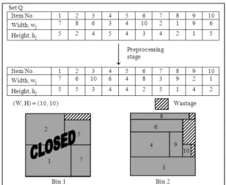
of two stages: preprocessing stage and packing stage. Preprocessing stage: The rectangles are sorted in increasing order of area (breaking ties by non-decreasing order of the differences between the width and the height). For instance, set Q:

{(7, 5), (8, 2), (6, 4), (3, 5), (4, 4), (10, 3), (2, 4), (1, 2), (9, 1), (6, 5)}

{(7, 5), (6, 5), (10, 3), (6, 4), (4, 4), (8, 2), (3, 5), (9, 1), (2, 4), (1, 2)}

after sorting. The preprocessing stage required O(nlogn) time.

Packing stage: The smallest dimension among the available rectangles in the list mini = 1,2,…j{wj,hj} (where

j = number of the remaining rectangles in the rectangles list) is stored. The value of minj{wj,hj} is updated after

the corresponding rectangle is packed.

At first, an empty bin is initialized as the current bin, the current point is at the bottom-left corner (x = 0, y = 0) and the current gap is the shortest edge between the height of the bin, H and the width of the bin, W. The first rectangle in the rectangles list is removed and placed at the bottom left of the current bin.

The pointer and the gap are updated as follow. The current point is the lowest and leftmost point of the current bin. The gap width is the difference between the x-coordinate and the right edge of the bin or the left edge of a tall rectangle while the height of gap is the difference between the y-coordinate and the height of the bin. The current gap is the shortest edge between the remaining gap height and gap width. The area of the current gap is also determined. Next, the rectangles list is examined again. If the current gap is less than the current value of minj{wj,hj}, then the

relevant space is regarded as the wastage. The pointer is raised to the next lowest and leftmost point where the corresponding current gap is at least as big as the value of minj{wj,hj}. If the current gap is the gap

width, then the rectangle with its width that can fill the gap completely is given priority to be chosen to be packed at the current point. If the current gap is the gap height, then the rectangle with its height that can fill the current gap completely is given the priority.

If there is no any rectangle that can fill the gap completely, the first rectangle in the list which its area is less than or equal to the area of the current gap and can fill the gap without overlapping with other rectangles that have been packed is selected to be placed at the current point. When the current bin is full or the pointer has been raised to the top of the current bin, the bin is closed. A new empty bin is initialized as the current bin and the process is continues until all the rectangles in the rectangles list are packed. Only one bin is opened at a time. This packing stage required O(n2) time. Figure 2 shows the LGFiOF by packing the set Q using two bins.

Computational experiments: The first set of experiment compares the different preordering sequences of the rectangles in the preprocessing stage of LGFi by using the lower bounds proposed by[2,5].

Fig. 2: Improved Lowest Gap Fill (LGFiOF) for

oriented case

Then, the LGFi is compared with some well known heuristic placement routines, namely BLF, LGF, FC and TP using the lower bounds proposed by[5].The LGFi is also compared with BLF and LGF where both routines required O(n2) time using lower bound proposed by Boschetti and Mingozzi[2]. In the oriented case, LGFiOF is

compared with AD and FC. All placement routines are coded in ANSI-C using Microsoft Visual C++ version 6.0 as the compiler. In this study we consider ten different classes of problems instances proposed in the literature. The first six classes (I-VI) are proposed by[1]. In each class all the items are generated in the same interval and are classified as follows:

Class I: wj and hj uniformly random in [1, 10],

W = H = 10

Class II: wj and hj uniformly random in [1, 10], W =

H = 30

Class III: wj and hj uniformly random in [1, 35], W =

H = 40

Class IV: wj and hj uniformly random in [1, 35], W =

H = 100

Class V: wj and hj uniformly random in [1, 100], W

= H = 100

Class VI: wj and hj uniformly random in [1, 100], W

= H = 300

The other four classes (VII-X) are introduced by Martello and Vigo[9] where a more realistic situation is considered. The items are classified into four types: Type 1: wj uniformly random in

2 W, W 3

 

 

 , hj

uniformly random in 1, H1 2

 

 

Type 2: wj uniformly random in

1 1, W

2

 

 

 , hj uniformly random in 2H, H

3

 

 

 .

Type 3: wj uniformly random in

1 W, W 2

 

 

 , hj

uniformly random in 1H, H 2

 

 

 .

Type 4: wj uniformly random in

1 1, W

2

 

 

 , hj uniformly random in 1, H1

2

 

 

 .

The bin size is W = H = 100 for all classes, while the items are as follow:

Class VII: Type 1 with probability 70%, Type 2, 3, 4 with probability 10% each.

Class VIII: Type 2 with probability 70%, Type 1, 3, 4 with probability 10% each.

Class IX: Type 3 with probability 70%, Type 1, 2, 4 with probability 10% each.

Class X: Type 4 with probability 70%, Type 1, 2, 3 with probability 10% each.

For each class, we consider five values of n: 20, 40, 60, 80 and 100, where n is the number of rectangles that need to be packed into the bins. For each combination of class and value of n, ten problem instances are generated. To investigate the best sorting procedure that gave LGFi better packing quality, different preordering sequences of the rectangles are tested in the preprocessing stage which is listed in Table 2.

The performance of the different preordering sequences of the rectangles and the various heuristic placement routines are compared on the basis of the average Ratio defined by:

10 _i

i i

1 UB

Average Ratio

10 LB

=

∑

where, UBi and LBi represent the heuristic solution and

the lower bound of the problem instance i respectively.

Table 2: Preordering sequences of the rectangles

Type of preordering sequences of the rectangles Notation Decreasing area (breaking ties by decreasing height) DA (DH) Decreasing area (breaking ties by decreasing width) DA (DW) Decreasing width (breaking ties by decreasing height) DW (DH) Decreasing height (breaking ties by decreasing width) DH (DW) Without preordering Random

RESULTS AND DISCUSSION

Table 3 and 4 show the computational results of LGFi with different preordering sequences of the rectangles in the preprocessing stage by using the lower bounds proposed by Dell’Amico et al.[5] and Boschetti and Mingozzi[2] respectively. Table 5 gives the comparison of five different heuristic placement routines namely BLF, LGF, FC, TP and LGFi using the lower bound proposed by Dell’Amico et al.[5] while Table 6 shows the comparison of LGFi with other two heuristic placement routines namely BLF and LGF where both routines required O(n2) time by using the lower bound proposed by Boschetti and Mingozzi[2]. Table 7 gives the comparison between the three different heuristic placement routines for oriented case of 2DBPP namely FC, AD and LGFiOF. For each type

of sorting in Table 3 and 4 as well as the different placement routines in Table 5-7, the entries report the average ratio, computed over ten problem instances. The final line for each class gives the average overall values over that class. The final line in all tables gives the overall average value over all classes. We do not give the execution time because it is negligible (never exceed 0.1 CPU sec).

From the overall average ratio of all classes in Table 3 and 4, we found that LGFi with DH(DW) preordering sequence gives the best solution quality. Therefore, in the preprocessing stage of LGFi, the rectangles are initially sorted in DH(DW). The computational results in Table 5 indicate that the LGFi produced a slightly better packing quality compared to LGF. However, neither of the placement routines for LGF, LGFi and TP can be classified as the clear winner in this experiment as they produced mixed degrees of success in each class. It is worth mentioning that TP has a time complexity of O(n3), while both LGF and LGFi has a time complexity of only O(n2). This shows that the LGFi is a more competitive heuristic placement routine.

Table 3: Comparison of different preordering sequences of the rectangles for LGFi using lower bound proposed by[5]

DA(DH) DA(DW) DW(DH) DH(DW) RANDOM Class I

20 1.030 1.030 1.050 1.040 1.080 40 1.050 1.050 1.060 1.050 1.080 60 1.060 1.060 1.060 1.060 1.110 80 1.060 1.060 1.060 1.060 1.120 100 1.030 1.030 1.030 1.030 1.070 Average 1.045 1.045 1.052 1.049 1.092

Class II

20 1.000 1.000 1.000 1.000 1.000 40 1.100 1.100 1.100 1.000 1.100 60 1.100 1.100 1.050 1.050 1.150 80 1.000 1.000 1.000 1.000 1.070 100 1.000 1.000 1.000 1.030 1.060 Average 1.040 1.040 1.030 1.017 1.075

Class III

20 1.110 1.110 1.180 1.130 1.200 40 1.120 1.120 1.150 1.120 1.220 60 1.100 1.100 1.110 1.110 1.230 80 1.090 1.090 1.120 1.100 1.220 100 1.070 1.080 1.090 1.090 1.190 Average 1.097 1.098 1.130 1.107 1.211

Class IV

20 1.000 1.000 1.000 1.000 1.100 40 1.000 1.000 1.100 1.000 1.100 60 1.100 1.100 1.100 1.100 1.250 80 1.070 1.070 1.100 1.030 1.100 100 1.030 1.030 1.030 1.030 1.100 Average 1.040 1.040 1.067 1.033 1.130

Class V

20 1.070 1.070 1.110 1.070 1.200 40 1.100 1.100 1.170 1.140 1.200 60 1.090 1.090 1.140 1.110 1.200 80 1.090 1.090 1.150 1.100 1.180 100 1.090 1.090 1.120 1.090 1.160 Average 1.087 1.087 1.136 1.100 1.186

Class VI

20 1.000 1.000 1.000 1.000 1.000 40 1.400 1.400 1.400 1.300 1.400 60 1.050 1.050 1.050 1.000 1.150 80 1.000 1.000 1.000 1.000 1.000 100 1.070 1.070 1.100 1.100 1.170 Average 1.103 1.103 1.110 1.080 1.143

Class VII

20 1.170 1.150 1.190 1.170 1.220 40 1.150 1.150 1.160 1.140 1.230 60 1.120 1.120 1.120 1.130 1.160 80 1.120 1.110 1.150 1.130 1.160 100 1.120 1.120 1.110 1.120 1.150 Average 1.135 1.129 1.146 1.138 1.182

Class VIII

20 1.150 1.150 1.190 1.170 1.270 40 1.180 1.180 1.160 1.170 1.240 60 1.110 1.110 1.120 1.120 1.140 80 1.120 1.120 1.140 1.130 1.160 100 1.100 1.100 1.110 1.100 1.150 Average 1.131 1.132 1.143 1.137 1.193

Class IX

20 1.010 1.010 1.020 1.000 1.010 40 1.020 1.020 1.020 1.010 1.020 60 1.010 1.010 1.010 1.010 1.010 80 1.010 1.010 1.010 1.010 1.010 100 1.010 1.010 1.010 1.010 1.010 Average 1.009 1.009 1.013 1.007 1.012

Class X

20 1.180 1.180 1.150 1.130 1.270 40 1.100 1.100 1.120 1.090 1.230 60 1.100 1.100 1.120 1.120 1.240 80 1.070 1.070 1.080 1.080 1.180 100 1.050 1.050 1.078 1.070 1.160 Average 1.099 1.099 1.105 1.098 1.216 Average 1.079 1.078 1.093 1.077 1.144

Table 4: Comparison of different preordering sequences of the rectangles for LGFi using lower bound proposed by[2]

DA(DH) DA(DW) DW(DH) DH(DW) RANDOM Class I

20 1.000 1.000 1.020 1.010 1.050 40 1.030 1.030 1.040 1.030 1.060 60 1.020 1.020 1.020 1.020 1.070 80 1.010 1.010 1.010 1.010 1.060 100 1.020 1.020 1.020 1.020 1.060 Average 1.014 1.014 1.021 1.018 1.060

Class II

20 1.000 1.000 1.000 1.000 1.000 40 1.100 1.100 1.100 1.000 1.100 60 1.100 1.100 1.050 1.050 1.150 80 1.000 1.000 1.000 1.000 1.070 100 1.000 1.000 1.000 1.030 1.060 Average 1.040 1.040 1.030 1.017 1.070

Class III

20 1.090 1.090 1.170 1.110 1.190 40 1.080 1.080 1.110 1.080 1.180 60 1.050 1.050 1.060 1.060 1.170 80 1.050 1.050 1.070 1.060 1.170 100 1.050 1.060 1.070 1.070 1.160 Average 1.064 1.065 1.095 1.073 1.174

Class IV

20 1.000 1.000 1.000 1.000 1.100 40 1.000 1.000 1.100 1.000 1.100 60 1.100 1.100 1.100 1.100 1.250 80 1.070 1.070 1.100 1.030 1.100 100 1.030 1.030 1.030 1.030 1.100 Average 1.040 1.040 1.067 1.033 1.130

Class V

20 1.030 1.030 1.070 1.030 1.150 40 1.050 1.050 1.120 1.090 1.140 60 1.060 1.060 1.110 1.080 1.170 80 1.040 1.040 1.100 1.050 1.130 100 1.060 1.060 1.090 1.060 1.130 Average 1.050 1.050 1.098 1.062 1.146

Class VI

20 1.000 1.000 1.000 1.000 1.000 40 1.400 1.400 1.400 1.300 1.400 60 1.050 1.050 1.050 1.000 1.150 80 1.000 1.000 1.000 1.000 1.000 100 1.070 1.070 1.100 1.100 1.170 Average 1.103 1.103 1.110 1.080 1.143

Class VII

20 1.170 1.150 1.190 1.170 1.220 40 1.150 1.150 1.160 1.140 1.230 60 1.120 1.120 1.120 1.130 1.160 80 1.110 1.110 1.150 1.130 1.160 100 1.110 1.110 1.110 1.110 1.140 Average 1.133 1.127 1.145 1.136 1.180

Class VIII

20 1.150 1.150 1.190 1.170 1.270 40 1.180 1.180 1.160 1.170 1.240 60 1.110 1.110 1.120 1.120 1.140 80 1.110 1.110 1.130 1.120 1.150 100 1.100 1.100 1.100 1.100 1.150 Average 1.128 1.129 1.140 1.134 1.190

Class IX

20 1.010 1.010 1.020 1.000 1.010 40 1.000 1.000 1.010 1.000 1.010 60 1.000 1.000 1.000 1.000 1.000 80 1.000 1.000 1.000 1.000 1.000 100 1.000 1.000 1.000 1.000 1.000 Average 1.002 1.002 1.007 1.000 1.005

Class X

Table 5: Comparison of BLF, LGF, FC, TP and LGFi routines using lower bound proposed by Dell’Amico et al.[5]

BLF LGF FC TP LGFi

Class I

20 1.090 1.030 1.060 1.050 1.040 40 1.120 1.040 1.080 1.060 1.050 60 1.130 1.050 1.090 1.050 1.060 80 1.150 1.060 1.090 1.060 1.060 100 1.120 1.040 1.070 1.030 1.030 Average 1.122 1.044 1.078 1.050 1.049

Class II

20 1.000 1.000 1.000 1.000 1.000 40 1.100 1.100 1.100 1.100 1.000 60 1.100 1.050 1.050 1.000 1.050 80 1.070 1.070 1.030 1.070 1.000 100 1.060 1.030 1.030 1.000 1.030 Average 1.065 1.050 1.042 1.034 1.017

Class III

20 1.200 1.060 1.180 1.060 1.130 40 1.220 1.130 1.160 1.110 1.120 60 1.260 1.100 1.190 1.110 1.110 80 1.270 1.100 1.150 1.100 1.100 100 1.230 1.080 1.130 1.080 1.090 Average 1.239 1.093 1.162 1.092 1.107

Class IV

20 1.000 1.000 1.000 1.000 1.000 40 1.000 1.000 1.000 1.000 1.000 60 1.100 1.150 1.100 1.100 1.100 80 1.100 1.100 1.100 1.070 1.030 100 1.130 1.070 1.070 1.030 1.030 Average 1.065 1.063 1.054 1.040 1.033

Class V

20 1.150 1.090 1.080 1.060 1.070 40 1.180 1.100 1.100 1.110 1.140 60 1.160 1.090 1.110 1.080 1.110 80 1.170 1.090 1.110 1.080 1.100 100 1.160 1.080 1.100 1.080 1.090 Average 1.165 1.092 1.100 1.082 1.100

Class VI

20 1.000 1.000 1.000 1.000 1.000 40 1.400 1.400 1.400 1.400 1.300 60 1.100 1.050 1.050 1.050 1.000 80 1.000 1.000 1.000 1.000 1.000 100 1.130 1.070 1.070 1.070 1.100 Average 1.127 1.103 1.104 1.104 1.080

Class VII

20 1.220 1.190 1.190 1.130 1.170 40 1.200 1.120 1.170 1.100 1.140 60 1.200 1.100 1.180 1.120 1.130 80 1.200 1.100 1.170 1.110 1.130 100 1.190 1.090 1.170 1.110 1.120 Average 1.202 1.119 1.176 1.114 1.138

Class VIII

20 1.230 1.150 1.160 1.160 1.170 40 1.220 1.160 1.190 1.160 1.170 60 1.190 1.090 1.180 1.110 1.120 80 1.190 1.100 1.160 1.110 1.130 100 1.190 1.090 1.170 1.120 1.100 Average 1.204 1.116 1.172 1.132 1.137

Class IX

20 1.010 1.010 1.000 1.010 1.000 40 1.020 1.020 1.010 1.020 1.010 60 1.010 1.010 1.010 1.010 1.010 80 1.010 1.010 1.010 1.010 1.010 100 1.010 1.010 1.010 1.010 1.010 Average 1.011 1.011 1.008 1.012 1.007

Class X

20 1.150 1.200 1.150 1.200 1.130 40 1.130 1.070 1.090 1.080 1.090 60 1.140 1.080 1.090 1.090 1.120 80 1.140 1.060 1.060 1.060 1.080 100 1.110 1.070 1.070 1.060 1.070 Average 1.135 1.098 1.092 1.098 1.098 Average 1.133 1.079 1.099 1.076 1.077

Table 6: Comparison of BLF, LGF and LGFi routines using lower bound proposed by Boschetti and Mingozzi[2]

LGFi LGF BLF LGFi LGF BLF

Class I Class VI

20 1.010 1.000 1.060 20 1.000 1.000 1.000 40 1.030 1.020 1.090 40 1.300 1.400 1.400 60 1.020 1.010 1.090 60 1.000 1.050 1.100 80 1.010 1.010 1.090 80 1.000 1.000 1.000 100 1.020 1.030 1.110 100 1.100 1.070 1.130 Average 1.018 1.012 1.089 Average 1.080 1.103 1.127

Class II Class VII

20 1.000 1.000 1.000 20 1.170 1.190 1.220 40 1.000 1.100 1.100 40 1.140 1.120 1.200 60 1.050 1.050 1.100 60 1.130 1.100 1.200 80 1.000 1.070 1.070 80 1.130 1.100 1.200 100 1.030 1.030 1.060 100 1.110 1.080 1.190 Average 1.017 1.050 1.065 Average 1.136 1.117 1.200

Class III Class VIII

20 1.110 1.040 1.190 20 1.170 1.150 1.230 40 1.080 1.090 1.180 40 1.170 1.160 1.220 60 1.060 1.050 1.210 60 1.120 1.090 1.190 80 1.060 1.060 1.230 80 1.120 1.090 1.180 100 1.070 1.060 1.210 100 1.100 1.090 1.190 Average 1.073 1.059 1.202 Average 1.134 1.113 1.201

Class IV Class IX

20 1.000 1.000 1.000 20 1.000 1.010 1.010 40 1.000 1.000 1.000 40 1.000 1.010 1.000 60 1.100 1.150 1.100 60 1.000 1.000 1.000 80 1.030 1.100 1.100 80 1.000 1.000 1.000 100 1.030 1.070 1.130 100 1.000 1.000 1.000 Average 1.033 1.063 1.065 Average 1.000 1.004 1.002

Class V Class X

20 1.030 1.050 1.110 20 1.100 1.180 1.130 40 1.090 1.050 1.130 40 1.090 1.070 1.130 60 1.080 1.070 1.130 60 1.120 1.080 1.140 80 1.050 1.050 1.120 80 1.080 1.060 1.140 100 1.060 1.060 1.140 100 1.070 1.070 1.110 Average 1.062 1.055 1.125 Average 1.093 1.093 1.130 Average 1.065 1.067 1.121

Table 7: Comparison of FC, AD and LDFiOF routines for oriented

case of 2DBPP

FC AD LDFiOF FC AD LDFiOF

Class I Class VI

20 1.120 1.120 1.110 20 1.000 1.000 1.000 40 1.080 1.090 1.060 40 1.400 1.400 1.400 60 1.070 1.070 1.050 60 1.100 1.050 1.100 80 1.060 1.060 1.040 80 1.000 1.000 1.000 100 1.060 1.050 1.030 100 1.1 1.070 1.100 Average 1.078 1.078 1.059 Average 1.12 1.104 1.120

Class II Class VII

20 1.100 1.000 1.000 20 1.08 1.100 1.100 40 1.100 1.100 1.100 40 1.09 1.100 1.070 60 1.100 1.100 1.100 60 1.07 1.070 1.040 80 1.070 1.070 1.030 80 1.06 1.060 1.060 100 1.030 1.030 1.030 100 1.04 1.040 1.030 Average 1.080 1.060 1.053 Average 1.068 1.074 1.059

Class III Class VIII

20 1.180 1.200 1.230 20 1.160 1.130 1.120 40 1.140 1.150 1.170 40 1.070 1.080 1.080 60 1.110 1.130 1.100 60 1.060 1.060 1.060 80 1.100 1.100 1.070 80 1.060 1.060 1.040 100 1.090 1.090 1.090 100 1.060 1.060 1.050 Average 1.124 1.134 1.131 Average 1.082 1.078 1.068

Class IV Class IX

Table 7: Continued

Class V Class X

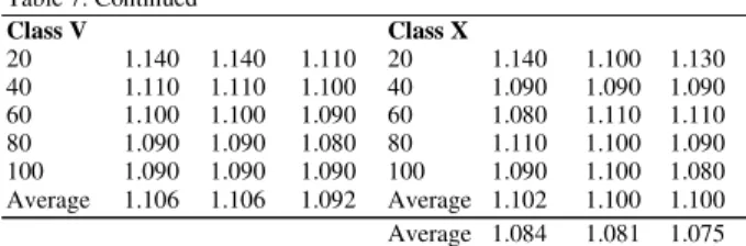
20 1.140 1.140 1.110 20 1.140 1.100 1.130 40 1.110 1.110 1.100 40 1.090 1.090 1.090 60 1.100 1.100 1.090 60 1.080 1.110 1.110 80 1.090 1.090 1.080 80 1.110 1.100 1.090 100 1.090 1.090 1.090 100 1.090 1.100 1.080 Average 1.106 1.106 1.092 Average 1.102 1.100 1.100 Average 1.084 1.081 1.075

In Table 7, the overall average ratio of all classes indicates that LGFiOF gives better packing quality if

compared to AD and FC. LGFiOF is also better than

AD and FC in terms of time complexity where both of AD and FC required O(n3) time while LGFiOF required

only O(n2) time.

CONCLUSION

In this study, we developed heuristics placement routines called the Improved Lowest Gap Fill, LGFi and LGFiOF for solving both non-oriented and oriented

cases of two-dimensional bin packing problems respectively. Both routines are capable of filling the available gaps in the partial layout by dynamically selecting the best rectangle for placement during packing stage. The routines require only O(n2) time. Computational results shown that our proposed routines are capable of producing high quality solution.

REFERENCES

1. Berkey, J.O. and P.Y. Wang, 1987. Two dimensional finite bin packing algorithms. J. Operat. Res. Soc., 38: 423-429. http://www.jstor.org/pss/2582731

2. Boschetti, M.A. and A. Mingozzi, 2003. The two- dimensional finite bin packing problem. Part II: New lower and upper bounds. 4OR: Q. J. Operat. Res. Soc., 1: 135-147. DOI: 10.1007/s10288-002-0006-y

3. Chazelle, B., 1983. The bottom-left bin packing heuristic: An efficient implementation. IEEE

Trans. Comput., 32: 697-707.

http://www2.computer.org/portal/web/csdl/doi/10.1 109/TC.1983.1676307

4. Coffman, E.G., M.R. Garey and D.S. Johnson, 1984. Approximation Algorithms for Bin Packing. In. Algorithm Design for Computer Systems Design, Ausiello, G., N. Lucertini and P. Seratini (Eds.). Springer, Vienna, ISBN: 0-387-81816-2, pp: 49-106.

5. Dell’Amico, M., S. Martello and D. Vigo, 2002. A lower bound for the non-oriented two-dimensional bin packing problem. Discrete Applied Math., 118: 13-24.

http://portal.acm.org/citation.cfm?id=584685.584688 6. Garey, M.R. and D.S. Johnson, 1979. Computer

and Intractability: A guide to the Theory of NP-Completeness. WH Freeman, San Francisco, ISBN: 0716710455, pp: 338.

7. Lee, L.S., 2008. A genetic algorithms for two-dimensional bin packing problem. MathDigest. Res. Bull. Inst. Math. Res., 2: 34-39.

8. Lodi, A., S. Martello and D. Vigo, 1999. Heuristic and metaheuristic approaches for a class of two-dimensional bin packing problems. INFORMS J.

Comput., 11: 345-357.

http://portal.acm.org/citation.cfm?id=768372 9. Martello, S. and D. Vigo, 1998. Exact solution of

the two-dimensional finite bin packing problem.

Manage. Sci., 44: 388-399.

http://portal.acm.org/citation.cfm?id=289228 10. Wäscher, G., H. Hauβner and H. Schumann, 2007.