www.hydrol-earth-syst-sci.net/19/4081/2015/ doi:10.5194/hess-19-4081-2015
© Author(s) 2015. CC Attribution 3.0 License.
Sensitivity of water scarcity events to ENSO-driven climate
variability at the global scale
T. I. E. Veldkamp1, S. Eisner2, Y. Wada3,4,5, J. C. J. H. Aerts1, and P. J. Ward1
1Institute for Environmental Studies (IVM), VU Amsterdam, Amsterdam, the Netherlands 2Center for Environmental Systems Research, University of Kassel, Kassel, Germany 3Center for Climate Systems Research, Columbia University, New York, USA 4NASA Goddard Institute for Space Studies, New York, USA
5Department of Physical Geography, Utrecht University, Utrecht, the Netherlands Correspondence to:T. I. E. Veldkamp ([email protected])
Received: 6 May 2015 – Published in Hydrol. Earth Syst. Sci. Discuss.: 11 June 2015 Revised: 4 September 2015 – Accepted: 28 September 2015 – Published: 8 October 2015
Abstract. Globally, freshwater shortage is one of the most dangerous risks for society. Changing hydro-climatic and socioeconomic conditions have aggravated water scarcity over the past decades. A wide range of studies show that water scarcity will intensify in the future, as a result of both increased consumptive water use and, in some regions, climate change. Although it is well-known that El Niño– Southern Oscillation (ENSO) affects patterns of precipitation and drought at global and regional scales, little attention has yet been paid to the impacts of climate variability on wa-ter scarcity conditions, despite its importance for adaptation planning. Therefore, we present the first global-scale sensi-tivity assessment of water scarcity to ENSO, the most domi-nant signal of climate variability.
We show that over the time period 1961–2010, both wa-ter availability and wawa-ter scarcity conditions are significantly correlated with ENSO-driven climate variability over a large proportion of the global land area (> 28.1 %); an area in-habited by more than 31.4 % of the global population. We also found, however, that climate variability alone is often not enough to trigger the actual incidence of water scarcity events. The sensitivity of a region to water scarcity events, expressed in terms of land area or population exposed, is determined by both hydro-climatic and socioeconomic con-ditions. Currently, the population actually impacted by wa-ter scarcity events consists of 39.6 % (CTA: consumption-to-availability ratio) and 41.1 % (WCI: water crowding in-dex) of the global population, whilst only 11.4 % (CTA) and 15.9 % (WCI) of the global population is at the same time
living in areas sensitive to ENSO-driven climate variabil-ity. These results are contrasted, however, by differences in growth rates found under changing socioeconomic condi-tions, which are relatively high in regions exposed to water scarcity events.
Given the correlations found between ENSO and water availability and scarcity conditions, and the relative devel-opments of water scarcity impacts under changing socioe-conomic conditions, we suggest that there is potential for ENSO-based adaptation and risk reduction that could be fa-cilitated by more research on this emerging topic.
1 Introduction
Haddeland et al., 2014; Kiguchi et al., 2015; Lehner et al., 2006; Prudhomme et al., 2014; Schewe et al., 2014; Sperna Weiland et al., 2012; Stahl, 2001; van Vliet et al., 2013; Wada et al., 2014a).
Whilst a wide range of studies have assessed the role of long-term climate change and changing socioeconomic conditions on past and future global blue water availabil-ity and water scarcavailabil-ity events, the impact of inter-annual cli-mate variability is less well understood (Kummu et al., 2014; Lundqvist and Falkenmark, 2010; Rijsberman, 2006; Veld-kamp et al., 2015). Taking into account the impact of climate variability relative to longer term changes in either the so-cioeconomic or climatic conditions is, however, important as these factors of change may amplify or offset each other at the regional scale (Hulme et al., 1999; McPhaden et al., 2006; Murphy et al., 2010; Veldkamp et al., 2015). Correct infor-mation on current and future water scarcity conditions and thorough knowledge of the relative contribution of its driv-ing forces, such as inter-annual variability, help water man-agers and decisions makers in the design and prioritization of adaptation strategies for coping with water scarcity.
To address this issue, we assess in this paper the sensitiv-ity of blue water resources availabilsensitiv-ity (i.e. the surface fresh water availability in rivers, lakes, wetlands, and reservoirs; Savenije, 2000; Wada et al., 2011b), consumptive water use, and blue water scarcity events to climate variability driven by El Niño–Southern Oscillation (ENSO) at the global scale over the time period 1961–2010. Moreover, we evaluated whether those areas with statistically significant correlations have been exposed to blue water scarcity events, if there is a spatial clustering in terms of population or land area exposed to blue water scarcity events and/or population living in ar-eas sensitive to ENSO-driven climate variability, and whether this spatial clustering has changed over time given the so-cioeconomic developments. Within this contribution we in-vestigate the impact of ENSO as it is the most dominant signal of inter-annual climate variability (McPhaden et al., 2006). Also, since ENSO can be predictable with reasonable skill up to several seasons in advance (Cheng et al., 2011; Ludescher et al., 2014), this can provide useful information for adaptation management to account for inter-annual vari-ability in blue water resources and blue water scarcity esti-mates, enabling the prioritization of adaptation efforts in the most affected regions ahead of those extreme events (Bouma et al., 1997; Cheng et al., 2011; Dilley and Heyman, 1995; Ludescher et al., 2013; Ward et al., 2014a, b; Zebiak et al., 2014).
ENSO is the result of a coupled climate variability sys-tem in which ocean dynamics and sea level pressure interact with atmospheric convection and winds (ocean–atmosphere feedback mechanisms). El Niño is the oceanic component, whereby waters over the eastern equatorial Pacific Ocean reach anomalously high temperatures. This eastern Pacific Ocean surface is relatively cool under neutral conditions, while it reaches anomalously low temperatures during La
Niña conditions. The Southern Oscillation is the atmospheric component, represented by the east–west shifts in the tropi-cal atmospheric circulation between the Indian and West Pa-cific oceans and the East PaPa-cific Ocean (Kiladis and Diaz, 1989; Parker et al., 2007; Rosenzweig and Hillel, 2008; Wal-lace and Hobbs, 2006; Wang et al., 2004). ENSO is well-known for its impacts on precipitation and hydrological ex-tremes (such as drought and flooding) at local and regional scales (e.g. Chiew et al., 1998; Kiem and Franks, 2001; Lü et al., 2011; Mosley, 2000; Moss et al., 1994; Piechota and Dracup, 1999; Räsänen and Kummu, 2013; Whetton et al., 1990; Zhang et al., 2015). Several studies have also examined ENSO’s impact at the global scale (Chiew and McMahon, 2002; Dai and Wigley, 2000; Dettinger et al., 2000; Dettinger and Diaz, 2000; Labat, 2010; Ropelewski and Halpert., 1987; Sheffield et al., 2008; Vicente-Serrano et al., 2011; Ward et al., 2010, 2014a). Though, only a limited number of stud-ies assessed the societal impacts (e.g. in terms of population affected, GDP loss, or with respect to human health) of hy-drological extremes under the different ENSO stages at the global scale (Bouma et al., 1997; Dilley and Heyman, 1995; Kovats et al., 2003; Rosenzweig and Hillel, 2008; Ward et al., 2014b). To the best of our knowledge, none of these studies have executed a global-scale assessment of the sensitivity of water resources availability, consumptive water use patterns, and water scarcity events to ENSO.
2 Methods
In short, we carried out this assessment through the fol-lowing steps: (1) used daily discharge and runoff time se-ries (0.5◦×0.5◦) from an ensemble of three global
hydro-logical models (WaterGAP, PCR-GLOBWB, and STREAM) (Sect. 2.1); (2) combined time series of water availability, consumptive water use, and population to calculate water scarcity conditions for the period 1961–2010 (Sect. 2.2–2.4); (3) identified statistical relationships between water avail-ability, consumptive water use and water scarcity conditions, and indices of ENSO (Sect. 2.5); and (4) evaluated whether the areas with significant correlations with ENSO are actu-ally affected by water scarcity events, how the impacts (pop-ulation and land area affected) are clustered, and how the impacts have changed through time (Sect. 2.5). Modelling uncertainty was evaluated by comparing the results from the ensemble-mean time series with the outcomes of the indi-vidual global hydrological models (Sect. 2.6). The following paragraphs describe our methods in detail.
2.1 Ensemble-mean monthly runoff and discharge We simulated global gridded daily discharge and runoff over the period 1960–2010 at a resolution of 0.5◦×0.5◦
al., 1999; Ward et al., 2007) and WaterGAP (Müller Schmied et al., 2014), forced with WATCH Forcing Data – ERA Interim (WFD-EI) daily precipitation and temperature data (0.5◦
×0.5◦) (Weedon et al., 2014) for the period 1979–
2010 and WATCH forcing data ERA40 (WFD) for the pe-riod 1960–1978 (Weedon et al., 2011). In order to compen-sate for offsets in long-term radiation fluxes between the two data sets, as found by Müller Schmied et al. (2014), WFD down-welling shortwave and long-wave radiation were ad-justed for use in WaterGAP to WFD-EI long-term means following the approach of Haddeland et al. (2012). Daily val-ues were aggregated to time series of monthly discharge and runoff. Using global hydrological models gives us the ad-vantage of a global coverage, whereas the portfolio of ob-served data sets (water availability and consumptive water use) is bounded by its biased regional distribution (Hannah et al., 2011; Ward et al., 2010, 2014a). However, we are aware of the caveats using these types of models to estimate water availability as all large-scale hydrological models have their own strengths and shortcomings (Gudmundsson et al., 2012; Nazemi and Wheater, 2015a, b). Therefore, we constructed ensemble-mean time series of both monthly discharge and runoff capturing the three global hydrological models. The results of the individual modelling efforts were used to eval-uate the modelling agreement (Sects. 2.4 and 3.5).
2.2 Calculating water availability
Water availability is expressed in this paper as the sum of monthly runoff per food producing unit (FPU). FPUs rep-resent a hybrid between river basins and economic regions for which it is generally assumed that water scarcity issues can be solved internally (Cai and Rosegrant, 2002; de Frai-ture, 2007; Kummu et al., 2010; Rosegrant et al., 2002). We used here an updated version of the FPU used by Kummu et al. (2010), which consists of 436 FPUs, excluding small is-land FPUs. For FPUs located within one of the world’s larger river basins, we redistributed runoff in order to avoid local over- or underestimations in water availability. Runoff was redistributed across the FPUs within these larger river basins, proportionally to the discharge distribution of that large river basin (Gerten et al., 2011; Schewe et al., 2014):
WAi= Rb∗Qi
P
Qi , (1)
whereby WAi is the monthly water availability within FPU i, Rbis the total monthly runoff within large river basinb, Qi
is the monthly discharge in FPUi, andPQiis the sum of the
monthly discharge over all cells within a large river basinb.
Subsequently, we calculated the annual water availabil-ity by aggregating the simulated ensemble-mean monthly water availability time series using hydrological years. The use of hydrological years is necessary in this assessment, as ENSO tends to develop to its fullest strength during the period December–February, which intersects with the
stan-dard calendar year boundaries (Ward et al., 2014a, b). Hy-drological years are referred to by the year in which they end, e.g. hydrological year 1961 refers here to the period October 1960–September 1961. Within this study we follow Ward et al. (2014a) and distinguish two hydrological years on the basis of long-term monthly maximum water availabil-ity per river basin: October–September (standard) and July– June (for river basins that have their long-term monthly max-imum water availability in September, October or Novem-ber). The river basin delineation used here was derived from the WATCH project (Döll and Lehner, 2002) and is equal to the river basin delineation that is used as the input for the FPU classification used within this study. We used the hy-drological years setting determined at grid level, using the WATCH river basins, as input for the distinction between hy-drological years at FPU scale. If an FPU consisted of more than one river basin we based the choice of hydrological year on the month (with long-term maximum water availability) with the highest prevalence within this FPU (see Supplement Fig. S1).
2.3 Calculating consumptive water use
Monthly gridded water consumption (0.5◦×0.5◦) was
esti-mated for the sectors livestock, irrigation, industry, and do-mestic within PCR-GLOBWB using daily WFD-EI precip-itation and temperature data in combination with yearly in-formation on livestock densities; the extent of irrigated areas; desalinated water use; non-renewable groundwater abstrac-tions; and past socioeconomic developments, namely GDP, energy and electricity production, household consumption, and population growth (Wada et al., 2011b, 2014b). For a complete description and extensive discussion of the method-ological steps taken to compose these monthly consumptive water use time series, we refer to Wada et al. (2011b, 2014b). Time series of desalinated water use and non-renewable groundwater abstractions were subtracted from the total con-sumptive water use estimates as they lower the need for blue water. Subsequently, we aggregated gridded monthly consumptive water use into yearly totals per FPU (WCi,yr),
2.4 Calculating water scarcity conditions
Blue water scarcity refers to the imbalance between blue wa-ter availability (i.e. wawa-ter in rivers, lakes, and aquifers) and the needs for water over a specific time period and for a certain region (Falkenmark, 2013). Although water scarcity could also relate to the green (water in the unsaturated soil), white (part of rainfall that feeds directly back into the at-mosphere), and deep blue (fossil groundwater) water sources (Savenije, 2000), we focus here on blue water scarcity (hereafter: water scarcity) only. Within this study we ap-plied two complementary indicators to express water scarcity conditions per FPU: the water crowding index (WCI) for population-driven water shortage and the consumption-to-availability ratio (CTA ratio) for demand-driven water stress (Brown and Matlock, 2011; Rijsberman, 2006). The WCI quantifies the yearly water availability per capita (Falken-mark et al., 1989, 2007; Falke(Falken-mark, 2013), whereby wa-ter demands are based on household, agricultural, industrial, energy, and environmental water consumption (Rijsberman, 2006). Like previous studies (e.g. Alcamo et al., 2007; Ar-nell, 2003; Kummu et al., 2010), we used 1700 m3capita−1
per year as the threshold level to evaluate water shortage events. The CTA ratio evaluates the ratio between consump-tive water used and water availability in a specific region and is a derivative from the withdrawal-to-availability (WTA; Raskin et al., 1997) ratio. Usually, a region is said to ex-perience water stress events when water withdrawals com-prises≥40 % of the available water resources, whilst
mod-erate water stress conditions occur if 20 %≥WTA≤40 %
(Raskin et al., 1997). The use of the WTA ratio is widely quoted and applied in previous research contributions, e.g. by Alcamo et al. (2003, 2007), Arnell et al. (1999), Cosgrove and Rijsberman (2000), Hanasaki et al. (2013), Kiguchi et al. (2015), Kundzewicz et al. (2007), Oki et al. (2001), Oki and Kanae (2006), and Vörösmarty et al. (2000). Hoekstra et al. (2012) and Wada et al. (2011a) applied this WTA ratio in an adapted form, using blue water footprints and potential consumptive water use estimates respectively to assess wa-ter stress conditions: the CTA ratio. This approach accounts for the share of water that has been recycled (industry) or not used (irrigation) and which flows back into the natural system. The threshold level for water stress using these con-sumptive water demands is therefore conceived to be lower than the threshold level for water stress as estimated using withdrawals. Following Hoekstra et al. (2011, 2012), Richter et al. (2011), and Wada et al. (2011a), we applied a thresh-old level of 0.2 to indicate water stress events. Equations (2) and (3) show the use of the WCI (WCIi,yr)and the CTA ratio
(CTAi,yr), respectively,
WCIi,yr=WAi,yr
Pi,yr
(water shortage event if WCIi,yr≤1700), (2)
CTAi,yr=WCi,yr
WAi,yr
(water stress event if CTAi,yr≥ 0.2),
(3) whereby WAi,yr is the water available per spatial uniti and
hydrological year yr,Pi,yr is the population, and WCi,yr is
consumptive water use. Water scarcity conditions were as-sessed here at the FPU scale. The FPU scale is seen as an appropriate spatial scale to study water scarcity conditions as it is generally assumed that lower-scale water scarcity issues can be overcome by the reallocation of water demand and supply within this spatial unit (Kummu et al., 2010). How-ever, one should keep in mind that, due to the assumption of full exchange possibilities – both from an infrastructural and water management perspective and its relative large spa-tial scale, analysis executed at the FPU scale may disguise lower-scale water scarcity issues (Kummu et al., 2010; Wada et al., 2011a).
The population data used for the calculation of the WCI (Eq. 2) were adopted from Wada et al. (2011a, b), who derived yearly gridded population maps (0.5◦×0.5◦) from
yearly country-scale FAOSTAT data in combination with decadal gridded global population maps (Klein Goldewijk and van Drecht, 2006). We aggregated these gridded popula-tion maps to FPU scale for use in this study. In line with the hydrological year naming convention, population estimates were used for the year in which the hydrological year ends; e.g. for hydrological year 1961 we used population estimates of 1961 as input for the WCI and to calculate water scarcity impacts.
2.5 Sensitivity of water availability, consumptive water use, and water scarcity conditions to ENSO
We examined the relationship respectively between water availability, consumptive water use, and water scarcity condi-tions, and ENSO-driven climate variability by means of their correlation with the Japan Meteorological Agency’s (JMA) Sea Surface Temperature (SST) anomaly index (http://coaps. fsu.edu/jma). We used here 3-monthly mean values of the JMA SST over the periods October–December, November– January, December–February, and January–March, as El Niño and La Niña expressions are strongest in these months (Dettinger and Diaz, 2000). Following Ward et al. (2014b), we examined the correlation between WAann,
WCann, CTAann, and WCIann, and the 3-monthly mean JMA
SST values (OND, NDJ, DJF, JFM), using Spearman’s rank correlation coefficient. Statistical significance was assessed by means of regular bootstrapping (n=1000, p≤0.05)
counted the number of individual tests with a significant re-sult and assessed the probability of yielding this rere-sult by chance given its statistical distribution (Livezey and Chen, 1982; Wilks, 2006). Subsequently, we examined the percent-age anomalies in the median values of water scarcity con-ditions between El Niño and La Niña years, compared to the median values under all years. To distinguish between El Niño, La Niña, and neutral years we used the classifica-tion of ENSO years from the Center for Ocean–Atmospheric Prediction Studies based on the JMA SST values. Years are assigned as El Niño or La Niña years when their 5-month moving average JMA SST index values are (±)0.5◦C or
greater (El Niño)/smaller (La Niña) for at least 6 consec-utive months (including October–December). Reference to the different ENSO years was adjusted to be consistent with the naming convention used for the hydrological years (Ta-ble 1). We used a bootstrapped version of the non-parametric Mann–WhitneyUtest (n=1000,p≤0.05) to test the
statis-tical differences in median values.
The critical threshold values put in place for the WCI and the CTA ratio (here 1700 and 0.2 respectively) determine whether water scarcity conditions adversely affect popula-tion or society. Per FPU we therefore evaluated which pro-portion of land area, for which we found a significant corre-lation between ENSO and water scarcity conditions, is also exposed to water scarcity events and how population is clus-tered in these areas compared to the general pattern of pop-ulation density. Moreover, we assessed how these numbers changed through time given the changing socioeconomic conditions, relative to developments in (1) the population and land area sensitive to ENSO-driven climate variability but not exposed to water scarcity events; (2) the population and land area exposed to water scarcity events in areas that lack a significant correlation with ENSO-driven climate variability; and to (3) the total population growth.
2.6 Evaluating modelling uncertainty
A cross-model validation was executed in order to evaluate the modelling uncertainty whereby we compared the results from the ensemble mean with the outcomes of the individual global hydrological models (GHM). We examined the agree-ment among the different modelling results and the ensem-ble mean when looking at (1) the sensitivity of water avail-ability and water scarcity conditions to ENSO-driven climate variability, and (2) the impacts of water scarcity events and relation to ENSO-driven climate variability under changing socioeconomic conditions.
3 Results
3.1 Sensitivity of water availability and consumptive water use to ENSO
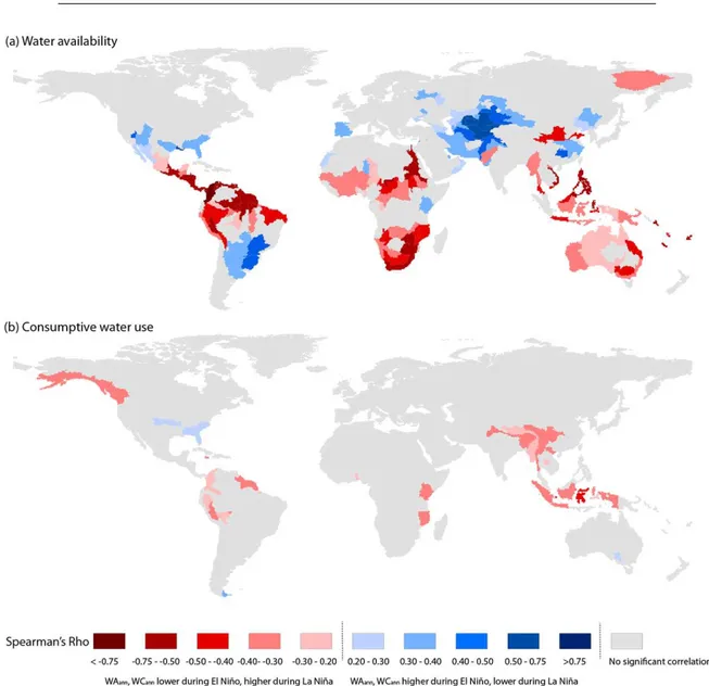
Significant correlations of water availability to variations in JMA SST were found across 37.1 % of the global land sur-face (excluding Greenland and Antarctica), whilst for con-sumptive water use (simulated under fixed socioeconomic conditions at 1961 levels) we found significant correlations covering 8.3 % of the total land area (Fig. 1 and Table 2). Using the 3-monthly JMA SST period with the highest cor-relation, Fig. 1 shows for both water availability and con-sumptive water use its correlation coefficient with the inter-annual variation in the 3-monthly average JMA SST val-ues. Only those correlations which reach statistical signifi-cance at a 95 % confidence interval are shown here. Field significance, the collectiveglobalsignificance of the total of individuallocal hypothesis tests (Livezey and Chen, 1982; Wilks, 2006), was tested for the individual 3-month correla-tion results and found to be highly significant when looking at water availability (p< 0.01) but insignificant when
consid-ering consumptive water use (p> 0.5). Positive correlations,
i.e. more water available with the JMA SST index moving towards El Niño values, were found for 13.2 % of the global land surface, while negative correlations were found in FPUs covering 23.9 % of the global land surface. When looking at consumptive water use we found positive significant correla-tions for only 1.0 %, and negative correlacorrela-tions for 7.3 % of the global land surface.
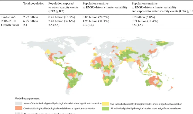
3.2 Sensitivity of water scarcity conditions to ENSO Subsequently, we assessed how sensitive water scarcity con-ditions (simulated under fixed socioeconomic concon-ditions at 1961 levels) are to ENSO-driven climate variability. Signif-icant correlations to variations in JMA SST were found for 28.1 and 37.9 % of the global land surface when using the CTA ratio (water stress) and WCI (water shortage) respec-tively, while being tested under a 95 % confidence interval (Table 3). Due to the clustering of population and consump-tive water use we found even higher percentages when look-ing at the population livlook-ing in these areas, 31.4 and 38.7 % of the global population in 2010 for the CTA ratio and WCI, respectively.
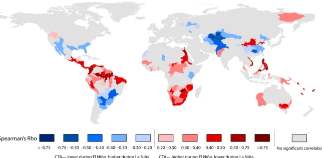
Figure 2 shows the areas with a significant positive (red) or negative (blue) correlation of water stress conditions (CTA ratio) with the variation in JMA SST values, using the 3-monthly JMA SST period with the highest correlation (JMA SSTbestoff). Correlation results found for water shortage
Table 1.Hydrological years that fall under the El Niño and La Niña phase. Other years are classified as ENSO neutral.
ENSO phase Hydrological year
El Niño 1964, 1966, 1970, 1973, 1977, 1983, 1987, 1988, 1992, 1998, 2003, 2007, 2010 La Niña 1965, 1968, 1971, 1972, 1974, 1975, 1976, 1989, 1999, 2000, 2008
Figure 1. Correlation (Spearman’s Rho) of yearly(a)water availability and(b)consumptive water use values, as assessed under fixed socioeconomic conditions, to variations in JMA SST using the 3-monthly period with the highest correlation (JMA SSTbestoff). Significance was tested by means of regular bootstrapping (n=1000,p≤0.05) and the correlation is only shown for those areas which reach significance. Positive correlations indicate increases in annual water availability and consumption with the JMA SSTbestoffindex moving towards El Niño values. Negative correlations indicate decreases in annual water availability with the JMA SSTbestoffindex moving towards El Niño values.
water scarcity conditions become more severe when the JMA SST index moves towards El Niño values (Table 3).
The regional variation in sensitivity of water scarcity con-ditions to ENSO-driven variability (Figs. 2 and S2) is clearly driven by the spatial distribution of water availability cor-relations as the general patterns are similar to those found in Fig. 1. The unequal clustering of water availability and
0.20 - 0.30
< -0.75 -0.75 - -0.50-0.50 - -0.40 -0.40- -0.30 -0.30 - 0.20 0.30 - 0.40 0.40 - 0.50 0.50 - 0.75 >0.75 No significant correlation
CTAann lower during El Niño, higher during La Niña CTAann higher during El Niño, lower during La Niña
Spearman’s Rho
Figure 2.Correlation (Spearman’s Rho) of yearly water scarcity conditions (CTA ratio), as assessed under fixed socioeconomic conditions, to variations in JMA SST using the 3-monthly period with the highest correlation (JMA SSTbestoff). Significance was tested by regular bootstrapping (n=1000, p≤0.05) and the correlation is only shown for those areas with significant correlations. Positive correlations indicate increases in CTA-ratio values (more severe water scarcity conditions) with the JMA SSTbestoff index moving towards El Niño values. Negative correlations indicate decreases in CTA-ratio values (less severe water scarcity conditions) with the JMA SSTbestoffindex moving towards El Niño values.
Table 2.Percentage of the global land area for which (a) water re-sources availability and (b) consumptive water use show a signifi-cant (positive/negative) correlation with ENSO-driven climate vari-ability (as assessed with the JMA SST anomaly index).
Significant Sign. positive Sign. negative correlation correlation correlation
Water availability 37.1 % 13.2 % 23.9 %
Consumptive water use 8.3 % 1.0 % 7.3 %
Table 3.Percentage of the global land area for which water scarcity conditions show a significant (positive/negative) correlation with ENSO-driven climate variability (as assessed with the JMA SST anomaly index). Water scarcity conditions were assessed by means of the CTA ratio for water stress and WCI ratio for water shortage.
Significant Sign. positive Sign. negative correlation correlation correlation Consumption-to-availability 28.1 % 16.8 % 11.3 % Ratio (CTA ratio)
Water crowding 37.9 % 23.9 % 14.0 %
Index (WCI)
water availability and consumptive water use, while they lack significant correlations when considering water stress con-ditions, and vice versa. In Southeast Asia, for example, we observed significant correlations between ENSO and water availability and consumptive water use (Fig. 1), but no sig-nificant correlations between ENSO and water stress (Fig. 2).
One explanation for this observation could be that if both water availability and consumptive water use increase or de-crease with more or less the same strength under changing JMA SST values, the net effect on the CTA ratio could be insignificant since the ratio between both variables remains equal. All FPUs that show a significant correlation between water resources availability and ENSO-driven climate vari-ability show as well a significant correlation with ENSO-driven variability when looking at the water shortage con-ditions (Fig. S2). This can be explained by the fact that the WCI is only driven by changes in water availability and pop-ulation growth, of which the latter factor was fixed in this analysis.
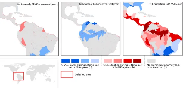
Subsequently, we assessed the percentage anomalies in the median values of water scarcity conditions between El Niño and La Niña years, compared to the median values under all years. Significant anomalies (p≤0.05, tested by
regu-lar bootstrappingn=1000) in water scarcity conditions
un-der El Niño and La Niña years, compared to all years, were found for 12.8 and 14.8 % of the global land area using the CTA ratio and the WCI, respectively (Table 4). The strongest anomaly signals were found during the La Niña phase for both water stress and shortage conditions.
CTAann higher during El Niño (a,c)
or La Niña years (b) CTAann lower during El Niño (a,c)
or La Niña years (b) No significant anomaly (a,b) or correlation (c)
Selected area
(a) Anomaly El Niño versus all years (b) Anomaly La Niña versus all years (c) Correlation JMA SSTbestoff
Figure 3.Comparison of results found when studying the(a)anomaly in water scarcity conditions (CTA ratio) between El Niño and all years, (b)anomaly in water scarcity conditions (CTA ratio) between La Niña and all years, and(c)the sensitivity of water scarcity conditions (CTA ratio) to ENSO-driven climate variability measured by means of the JMA SSTbestoff. Red colours indicate more severe scarcity conditions under El Niño phases(a, c)or La Niña phases(b). Blue colours indicate less severe scarcity conditions under El Niño phases(a, c)or La Niña phases(b).
(a) Population exposed (b) Land area exposed
Not exposed to water scarcity; Sensiive to ENSO driven variability Exposed to water scarcity; Not sensiive to ENSO driven variability Total populaion growth/land area
Exposed to water scarcity; Sensiive to ENSO driven variability
0 50 100 150 200 250
0 50 100 150 200 250
1961 1971 1981 1991 2001 2010 1961 1971 1981 1991 2001 2010
P
o
pul
a
ti
o
n
(%, Total Pop. 1
9
6
1
=
1
0
0
)
Land Area (%)
Figure 4.Development of population and land area exposed to water scarcity events and/or being sensitive to ENSO-driven climate variability over the period 1961–2010, as estimated with the CTA ratio.(a)shows the growth in population living under water scarce conditions and/or living in areas sensitive to ENSO-driven climate variability relative to the total growth in global population (set at 100 in 1961).(b)shows the increase in land area exposed to either water scarcity events and/or ENSO-driven climate variability relative to the total global land area (100).
show significant anomalies when looking at the different ENSO phases. This can be explained by the fact that only those years for which the 5-month moving average JMA SST index values are (±)0.5◦C or greater (El Niño)/smaller (La
Niña) for at least 6 consecutive months (including October– December) are assigned as El Niño or La Niña years (see Sect. 2.5). Using this ENSO year definition thus disguises all variability in JMA SST values that falls just below the threshold set; i.e. variation that can have, however, a signifi-cant effect on water scarcity conditions.
3.3 Sensitivity of water scarcity events to ENSO under changing socioeconomic conditions
West & Central Asia
Middle East
Not exposed to water scarcity; Sensiive to ENSO driven variability Exposed to water scarcity; Not sensiive to ENSO driven variability Total populaion growth
Exposed to water scarcity; Sensiive to ENSO driven variability
Latin America Caribbean
Northern America
Australia & Pacific Southeast Asia
East Asia (China)
South Asia (India)
Middle & Southern Africa Northern Africa
Western Europe
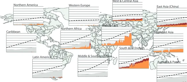
Figure 5.Regional variation in developments of population (%) exposed to water scarcity events and/or being sensitive to ENSO-driven climate variability over the period 1961–2010, as estimated with the CTA ratio. The figure shows per world region the growth in population living under water scarcity conditions and/or living in areas sensitive to ENSO-driven climate variability, relative to the total growth in global population (set at 100 in 1961).Yaxis (% population) ranges from 0 up to 400.
Table 4.Percentage of the global land area for which FPUs show significant anomalies in the median values of water scarcity condi-tions between the El Niño (EN) and La Niña (LN) phase, compared to the median values under all years. Water scarcity conditions were assessed by means of the CTA ratio for water stress and WCI ratio for water shortage.
Significant Sign. anomaly Sign. anomaly anomaly – El Niño phase – La Niña phase
Consumption to 12.8 % 3.4 % 12.8 %
availability Ratio (CTA ratio)
Water crowding 14.8 % 6.9 % 9.5 %
Index (WCI)
of 2.4 over the same time period whilst its proportion to the global total population remained relatively unchanged (Ta-ble 5). The population sensitive to ENSO variability and liv-ing in areas exposed to water scarcity events currently repre-sent only a minority of the global population (11.4 %). These results are, however, contrasted with relative high growth fac-tors (Table 5). The impact the spatial clustering of population and consumptive water use, and their unequal growth rates, on water scarcity events is shown by the fact that the share of land area exposed to water scarcity events only doubled over this same period for the CTA ratio (Fig. 4), from 7.4 up to 16.5 % of the global land surface . The results found for wa-ter shortage (WCI≤1700) are roughly similar at the global
scale (Supplement Fig. S3, Table S1) and therefore not dis-cussed individually in this section.
Regional variations in the population exposed to water stress and/or being sensitive to ENSO-driven climate vari-ability under changing socioeconomic conditions, are visu-alized in Fig. 5. Although these regional figures do not lend themselves to a similar growth factor analysis, such as ex-ecuted on the global numbers in Fig. 4, we can distinguish by means of visual inspection different characteristic region types. The first group of regions (Latin America Australia and the Pacific, the Caribbean, and Middle and Southern Africa) experiences significant correlations with ENSO vari-ability for a relative large share of its land area and popula-tion (≥25 % of the total population in 2010) whilst exposure
to water scarcity events is low (< 25 % of the total population in 2010). The second group of regions shows both a relatively low sensitivity to ENSO-driven climate variability (< 25 % of the total population in 2010) and low exposure to water scarcity events (< 25 % of the total population in 2010), e.g. northern America and western Europe. For the third group of regions (the Middle East, India, Southeast Asia, and western and central Asia) we find significant water scarcity exposure (≥25 % of the total population in 2010) but no or relative low
sensitivity to ENSO variability (< 25 % of the total popula-tion in 2010). Finally, the fourth group of regions shows rel-atively high exposure to water scarcity events (≥25 % of the
total population in 2010) and abundant sensitivity to ENSO-driven climate variability (≥25 % of the total population in
Table 5.Development of (a) the global total population, (b) the global population exposed to water scarcity events (CTA ratio), (c) the global population living in areas sensitive to ENSO-driven climate variability, and (d) the global population being exposed to water scarcity events (CTA ratio) and living in areas sensitive to ENSO-driven climate variability, between 1961 and 2010 using 5-year averaged values. Numbers between brackets show the values expressed in percentage of the total population. Growth factors represent both the absolute increases as well as the relative increases over time.
Total population Population exposed Population sensitive Population sensitive
to water scarcity events to ENSO-driven climate variability to ENSO-driven climate variability
(CTA≥0.2) and exposed to water scarcity events (CTA≥0.2)
1961–1965 2.97 billion 0.45 billion (15.3 %) 0.85 billion (28.7 %) 0.2 billion (6.8 %) 2006–2010 6.25 billion 2.48 billion (39.6 %) 1.96 billion (31.3 %) 0.71 billion (11.4 %)
Growth factor 2.1 5.5 (2.6) 2.3 (0.4) 3.5 (1.5)
Modelling agreement
None of the individual global hydrological models show significant correlation
One individual global hydrological model shows a significant correlation
Two individual global hydrological models show a significant correlation
All individual global hydrological models show a significant correlation
The ensemble-mean shows a significant correlation
Figure 6.Modelling agreement in observed significant sensitivity of water availability to variation in JMA SST.
Asia (relative high sensitivity to ENSO variability and rela-tive low water scarcity exposure), and middle and southern Africa, the Middle East and Southeast Asia (both experienc-ing relative high sensitivity to ENSO variability and high ex-posure to water scarcity events). Using both water scarcity metrics (i.e. CTA ratio and WCI) in combination with the observed growth rates in population and population exposed to water scarcity events enables us to identify those regions where adaptation measures, such as ENSO-based forecast-ing, have the largest (future) potential in coping with and pos-sibly reducing the adverse impacts of water scarcity events: the Caribbean, Latin America, western and central Asia, mid-dle and southern Africa, northern Africa, the Midmid-dle East, China, Southeast Asia and Australia, and the Pacific.
3.4 Cross-model validation
The cross-model validation exercise, in which we compared the outcomes of the individual global hydrological models with their ensemble-mean results, reveals that our findings considering the sensitivity of water availability, consumptive
water use, and water scarcity conditions to ENSO-driven cli-mate variability are robust in comparison to the use of dif-ferent hydrological models. We found that for 22.8 % of the global land area (61.4 % of the total land area with a sig-nificant correlation under the ensemble mean) all individual GHMs show a significant correlation to variations in JMA SST in the same direction as the correlation results found under the ensemble means. Correlations found under the en-semble mean are supported by at least one of the global hy-drological models for one-third (36.8 %) of the global land surface (Fig. 6), equal to 99.2 % of the land area that shows a significant correlation to the ensemble mean.
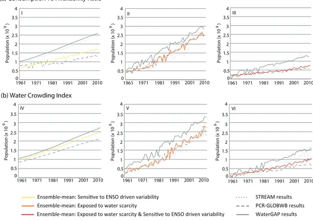
STREAM results
PCR-GLOBWB results
WaterGAP results Ensemble-mean: Sensiive to ENSO driven variability
Ensemble-mean: Exposed to water scarcity
Ensemble-mean: Exposed to water scarcity & Sensiive to ENSO driven variability
0 0.5 1 1.5 2 2.5 3 3.5 4 P o p u lat io
n (x 10 )
9 0 0.5 1 1.5 2 2.5 3 3.5 4 P o p u lat io
n (x 10 )
9
1961 1971 1981 1991 2001 2010 1961 1971 1981 1991 2001 2010 II I III 0 0.5 1 1.5 2 2.5 3 3.5 4 P o p u lat io
n (x 10 )
1961 1971 1981 1991 2001 2010
9
(a) Consumption To Availability Ratio
(b) Water Crowding Index
0 0.5 1 1.5 2 2.5 3 3.5 4 P o p u lat io
n (x 10 )
9 0 0.5 1 1.5 2 2.5 3 3.5 4 P o p u lat io
n (x 10 )
9 0 0.5 1 1.5 2 2.5 3 3.5 4 P o p u lat io
n (x 10 )
9
1961 1971 1981 1991 2001 2010 1961 1971 1981 1991 2001 2010
1961 1971 1981 1991 2001 2010
VI V
IV
Figure 7. Development of the population exposed to water scarcity events (CTA ratio) and/or being sensitive to ENSO-driven climate variability over the period 1961–2010, as assessed by the individual global hydrological models (STREAM, PCR-GLOBWB, and WaterGAP) and the ensemble mean.(I)and(IV)show the development in population sensitive to ENSO-driven climate variability as estimated under the ensemble-mean (yellow) and individual GHMs (grey).(II)and(V)present the increase in population exposed to water scarcity events for the ensemble-mean (orange) and individuals GHMs (grey).(III)and(VI)visualize the amount of people being exposed to water scarcity events, while at the same time living in areas with a significant correlation to ENSO-driven climate variability for the ensemble-mean (red) and individual GHMs (grey).
largest variations when looking at the population both being exposed to water scarcity events and living in areas sensi-tive to ENSO-driven climate variability (+68.9 % CTA
ra-tio,+54.2 % WCI). Percentage deviations were found to be
smaller when looking at the land area exposed (Supplement Fig. S5). As shown in Fig. 7 and Fig. S5, the inter-model comparison reveals that the impact estimates of the ensem-ble mean are conservative when comparing them with the individual modelling results, especially when looking at the population or land area sensitive to ENSO variability and/or being exposed to water scarcity events.
4 Discussion
Within this study we found that both water resources avail-ability and water scarcity conditions can be significantly cor-related with ENSO-driven climate variability as measured with the JMA SST index for a relatively large share of the global land area. Due to clustering effects we found even larger proportions when looking at the population living in these areas.
ENSO and the natural variability in the flow of tropical rivers. Significant correlations as shown for other regions were also found in case studies focusing on northern America (e.g. Clark II et al., 2014; Schmidt et al., 2001), Southeast Asia (e.g. Lü et al., 2011; Räsänen and Kummu, 2013), southern Africa (e.g. Meque and Abiodun, 2014; Richard et al., 2001), and Australia (e.g. Chiew et al., 2011; Dutta et al., 2006). The spatial variation in the sign of the found correlation is in line with the results of Ward et al. (2014a), who found that annual flood and mean discharge values intensify under La Niña and decline when moving towards El Niño phases globally in more areas than the other way around.
In line with earlier research (e.g. Meza et al., 2005; Islam and Gan, 2015) we would have expected to find more ar-eas with a significant correlation between consumptive wa-ter use and ENSO-driven climate variability. A number of explanations could be given for the absence of significant correlations patterns in this study: (1) the consumptive wa-ter use estimates used in this study are calculated by means of multiple socioeconomic and hydro-climatic proxies and variables, such as extent of irrigated areas, number of live-stock, GDP, (long-term mean) monthly temperatures, and precipitation estimates, and should be interpreted as poten-tial consumptive water use; (2) of these variables only irri-gation water use could be linked directly to ENSO-driven climate variability by means of its temperature and precipi-tation input variables. Fixed consumption numbers in other sectors might attenuate therefore the variability found within the irrigation sector; (3) yearly totals of consumptive wa-ter use were applied in this study to assess its sensitivity to ENSO-driven climate variability whereas it might be more appropriate for consumptive water use to assess its correla-tion either using monthly timescales or yearly maxima; and (4) climate-driven variations in irrigation water demands are the result of changes in crop evapotranspiration and changes in green water availability, which do not have a unequivocal relation with ENSO-driven climate variability at all times, but are partly determined by the month-specific cropping cal-endar and antecedent conditions, such as the memory of the soil. Soil memory is often referred to as the persistence of the soil to anomalous wet or dry conditions long after these conditions occurred in the atmosphere or any other stage of the hydrological cycle which could lead to time lags and attenuation of the meteorological signal (Seneviratne et al., 2006; Liu and Avissar, 1999). The found variability in the irrigation water demand estimates might, therefore, be out of phase with the variability found in the atmospheric con-ditions (ENSO-driven climate variability as assessed by the JMA SST anomaly index) which, in turn, explains the rela-tive low significant correlation. Including, per region or soil characteristic area, the size of the soil memory as a time lag could potentially improve the correlation of consumptive (ir-rigation) water demand with ENSO-driven climate variabil-ity. More research is, however, needed in order to be able to
express this relation between the size of the soil memory and the time lag used within the ENSO correlation analysis.
The analysis presented in this study revealed that inter-annual variability itself, such as the ENSO-driven climate variability, is often not enough to cause water scarcity events to actually occur. We found that it is a combination of multi-ple hydro-climatic factors, such as the mean water resources availability and its inter-annual variability around the mean, together with the prevalent socioeconomic conditions, that determines the susceptibility of a region to water scarcity events, a finding earlier suggested by Veldkamp et al. (2015) and Wada et al. (2011a), and its implications being discussed in Hall and Borgomeo (2013). The actual impact of water scarcity events depends, moreover, not only on the number of people exposed or the severity of a water scarcity event itself, but on how sensitive this population is to water scarcity con-ditions, whether and how efficiently governments can deal with water scarcity problems, and how many (financial and infrastructural) resources are available to cope with these wa-ter scarce conditions (Grey and Sadoff, 2007; Hall and Bor-gomeo, 2013).
Given the substantial share of land area, and the even higher rates of population, for which water resources avail-ability and water scarcity conditions show significant corre-lations with ENSO-driven climate variability there is a large potential for ENSO-based adaptation and risk reduction to cope with water scarcity events and their associated impacts. The relative importance of ENSO-driven climate variability in the year-to-year-variability as found in this study could assist water managers and decisions makers in the design of adaptation strategies, such as in optimizing the use of ex-isting reservoir facilities in Australia (Sharma, 2000). More-over, the potential predictability of ENSO, with lead times up to several months, may help in the prioritization of (ex ante) efforts in disaster risk reduction, such as pre-stocking foods and disaster relief goods or crop insurance systems based on ENSO indices (Coughlan de Perez et al., 2014, 2015; Dil-ley, 2000; Suarez et al., 2008). The potential added value of adaptation measures targeted towards mitigating the im-pacts of inter-annual variability is high, as it is especially this variability that people find difficult to cope with (Smit and Pilifosova, 2003). In this paper we looked, however, at nat-uralized flows, so reservoirs or inter-basin transfers have not yet been taken into account. Future research should there-fore, first evaluate whether (virtual) water trading and water storage mechanisms are effective in reducing water scarcity conditions and whether management could be optimized us-ing ENSO-forecastus-ing parameters and at what costs.
ex-treme ENSO events may become more frequent in the future (Cai et al., 2014; IPCC, 2013; Power et al., 2013). The uncer-tainty among the different climate models is, however, large and at the same time there is no agreement yet on the attri-bution of long-term climate change to increases in the sen-sitivity and frequency of ENSO events (van Oldenborgh et al., 2005; Paeth et al., 2008; Guilyardi et al. 2009). Consid-ering a continuous increase in population growth and water scarcity impacts in the future, hotspots could be identified that have to deal with water scarcity events and are sensi-tive to ENSO-driven variability at the same time. One should take into account, however, that we assumed in this study that the correlations found between water availability, con-sumptive water use, and water scarcity conditions, and the JMA SST index value remain stationary over time. In real-ity, the strength of correlations between hydrological param-eters and ENSO can change over time (Ward et al., 2014a). Further research is therefore needed to assess whether, how much, and in which direction these observed correlation values change under the combination of changing climatic conditions and historic and future socioeconomic develop-ments. Moreover, ENSO is part of an ocean–atmospheric climate variability system that constitutes many more sub-regional systems and local circulation patterns (e.g. Indian monsoon, Pacific/North America pattern, North Atlantic Os-cillation, East Atlantic/West Russia pattern, Scandinavia pat-tern) which modulate the ENSO signal (Hannaford et al., 2011). Future research should look into the sensitivity of wa-ter resources availability and scarcity conditions to combina-tions of these systems.
Global assessment studies, such as the one presented here, are well able to identify the impact of ENSO on global-scale patterns of water scarcity. These types of studies are there-fore well-suited for a first-order problem definition or for the large-scale prioritization of adaptation efforts. When inter-preting these assessments one should keep in mind, however, that these studies should always be complemented with local or regional-scale analyses to assess the actual level of wa-ter scarcity on the ground, their (economic) consequences, and regional or local-scale potential for ENSO forecasting as adaptation strategy to cope with water scarcity events.
5 Conclusions
Within this contribution, we executed the first global-scale sensitivity assessment of blue water availability, consump-tive water use, and water scarcity to ENSO-driven climate variability. Throughout this paper we have shown that re-gional water scarcity conditions become more extreme under El Niño and La Niña phases covering a relative large pro-portion (> 28.1 %) of the global land area. Due to the spa-tial clustering of population and consumptive water use we found even larger shares (> 31.4 % of the total population in 2010) when looking at the population living in these
ar-eas being sensitive to ENSO-driven climate variability. The exposure of a region to water scarcity events is determined by both hydro-climatic and socioeconomic conditions. Re-sults on exposure to water scarcity events, found in this study, provide mixed signals. We found that the population that is currently exposed to water scarcity events consists of less than half of the global population (CTA ratio: 39.6 %; WCI: 41.1 %), whilst the population sensitive to ENSO variability and living in areas exposed to water scarcity events represent only a minority of the global population (CTA ratio: 11.4 %; WCI: 15.9 %). These results are, however, contrasted by rel-ative differences in growth rates under changing socioeco-nomic conditions, which are higher in regions exposed to wa-ter scarcity events than in regions that do not experience any water scarcity.
Given the correlations found in this study for water avail-ability and water scarcity conditions with ENSO-driven cli-mate variability, and having seen the developments in the population and land area exposed to water scarcity events and/or being sensitive to ENSO-driven variability under changing socioeconomic conditions, we found that there is large potential for ENSO-based adaptation and risk reduc-tion. The observed regional variations could thereby accom-modate in a first-cut prioritization for such adaptation strate-gies. Moreover, the results presented in this study show that there is both potential and need for more research on the is-sue of ENSO and water scarcity with emerging topics related to the economic impacts of water scarcity, the assessment of consumptive water use and its temporal variability, the com-bined impact of large-scale oscillation systems on water re-sources and water scarcity conditions, and the transferability of global-scale insights to local-scale implications and deci-sions.
The Supplement related to this article is available online at doi:10.5194/hess-19-4081-2015-supplement.
Author contributions. T. I. E. Veldkamp, J. C. J. H. Aerts, and P. J. Ward designed research; T. I. E. Veldkamp, S. Eisner and Y. Wada prepared data sets; T. I. E. Veldkamp analyzed data; and T. I. E. Veldkamp, S. Eisner, Y. Wada, J. C. J. H. Aerts, and P. J. Ward wrote the paper.
Research Fellowship (grant no. JSPS-2014-878). P. Ward received funding from the Netherlands Organisation for Scientific Research (NWO) in the form of a VENI grant (grant no. 863-11-011).
Edited by: J. Hannaford
References
Aerts, J. C. J. H., Kriek, M., and Schepel, M.: STREAM (Spatial Tools for River Basins and Environment and Analysis of Man-agement Options): “Set Up and Requirements.”, Phys. Chem. Earth Pt. B, 24, 591–595, 1999.
Alcamo, J., Döll, P., Kaspar, F., and Siebert, S.: Global change and global scenarios of water use and availability: An Application of WaterGAP1.0, University of Kassel, Germany, p. 47, 1997. Alcamo, J., Döll, P., Henrichs, T., Kaspar, F., Lehner, B.,
Rösch, T., and Siebert, S.: Global estimates of water withdrawals and availability under current and future “business-as-usual” conditions, Hydrolog. Sci. J., 48, 339– 348, doi:10.1623/hysj.48.3.339.45278, 2003.
Alcamo, J., Flörke, M., and Märker, M.: Future long-term changes in global water resources driven by socioeco-nomic and climatic changes, Hydrolog. Sci. J., 52, 247–275, doi:10.1623/hysj.52.2.247, 2007.
Amarasekera, K. N., Lee, R. F., Williams, E. R., and Eltahir, E. A. B.: ENSO and the natural variability in the flow of tropical rivers, J. Hydrol., 200, 24–39, doi:10.1016/S0022-1694(96)03340-9, 1997.
Arnell, N. W.: Climate change and global water resources, Environ-mental Change, 9, S31–S49, 1999.
Arnell, N. W.: Effects of IPCC SRES* emissions scenarios on river runoff: a global perspective, Hydrol. Earth Syst. Sci., 7, 619–641, doi:10.5194/hess-7-619-2003, 2003.
Bouma, M. J., Kovats, R. S., Goubet, S. A., Cox, J. S. H., and Haines, A. T.: Global assessment of El Niño ’ s disaster burden, The Lancet, 350, 1435–1438, 1997.
Brown, A. and Matlock, M. D.: A Review of Water Scarcity Indices and Methodologies, The Sustainabil-ity Consortium White paper (No. 106), UniversSustainabil-ity of Arkansas, http://www.sustainabilityconsortium.org/wp-content/themes/sustainability/assets/pdf/whitepapers (last access: 7 October 2015), 21 pp., 2011.
Cai, W., Borlace, S., Lengaigne, M., van Rensch, P., Collins, M., Vecchi, G., Timmermann, A., Santoso, A., McPhaden, M.J., Wu, L., England, M. H., Wang, G., Guilyardi, E., and Jin, F.-F.: Increasing frequency of extreme El Niño events due to greenhouse warming, Nature Climate Change, 4, 111–116, doi:10.1038/nclimate2100, 2014.
Cai, X. M. and Rosegrant, M. W.: Global Water De-mand and Supply Projections, Water Int., 27, 159–169. doi:10.1080/02508060208686989, 2002.
Cheng, Y., Tang, Y., and Chen, D.: Relationship between pre-dictability and forecast skill of ENSO on various time scales, J. Geophys. Res., 116, C12006, doi:10.1029/2011JC007249, 2011. Chiew, F. H. S. and McMahon, T. A.: Global ENSO-streamflow teleconnection, streamflow forecasting and interannual variability, Hydrolog. Sci. J., 47, 505–522, doi:10.1080/02626660209492950, 2002.
Chiew, F. H. S., Piechota, T. C., Dracup, J. A., and McMahon, T. A.: El Nino Southern Oscillation and Australian rainfall, streamflow and drought: Links and potential for forecasting, J. Hydrol., 204, 138–149, doi:10.1016/S0022-1694(97)00121-2, 1998.
Chiew, F. H. S., Young, W. J., Cai, W., and Teng, J.: Current drought and future hydroclimate projections in southeast Australia and implications for water resources management, Stoch. Env. Res. Risk A., 25, 601–612, doi:10.1007/s00477-010-0424-x, 2011. Clark II, C., Nnaji, G. A., and Huang, W.: Effects of f El-Niño and a
La-Niña Sea Surface Temperature Anomalies on Annual Precipi-tations and Streamflow Discharges in Southeastern United States, J. Coastal Res., 68, 113–120, doi:10.2112/SI68-015.1, 2014. Cosgrove, W. and Rijsberman, F.: World water vision: Making
wa-ter everybody’s business, Earthscan, London, 2000.
Coughlan de Perez, E., Monasso, F., van Aalst, M., and Suarez, P.: Science to prevent disasters, Nat. Geosci., 7, 78–79, doi:10.1038/ngeo2081, 2014.
Coughlan de Perez, E., van den Hurk, B., van Aalst, M. K., Jong-man, B., Klose, T., and Suarez, P.: Forecast-based financing: an approach for catalyzing humanitarian action based on extreme weather and climate forecasts, Nat. Hazards Earth Syst. Sci., 15, 895–904, doi:10.5194/nhess-15-895-2015, 2015.
Dai, A. and Wigley, T. M. L.: Global patterns of ENSO-induced precipitation, Geophys. Res. Lett., 27, 1283–1986, doi:10.1029/1999GL011140, 2000.
De Fraiture, C.: Integrated water and food analysis at the global and basin level. An application of WATERSIM, Water Resour. Manag., 21, 185–198, doi:10.1007/s11269-006-9048-9, 2007. Dettinger, M. D. and Diaz, H. F.: Global Characteristics of Stream
Flow Seasonality and Variability, J. Hydrometeorol., 1, 289–310, 2000.
Dettinger, M. D., Cayan, D. R., Mccabe, G. J., and Marengo, J. A.: Multiscale streamflow variability associated with El Niño/Southern Oscillation, in: El Nino and the Southern Oscil-lation – Multiscale Variability and Global and Regional Impacts, Cambridge University Press, Cambridge, 113–146, 2000. Dilley, M.: Reducing vulnerability to climate variability in
South-ern Africa: The growing role of climate information, Climatic Change, 45, 63–73, 2000.
Dilley, M. and Heyman, B. N.: ENSO and Disaster: Droughts, Floods and El Nino/Southern Oscillation warm Events, Disas-ters, 19, 181–193, 1995.
Döll, P. and Lehner, B.: Validation of a new global 30-min drainage direction map, J. Hydrol., 258, 214–231, doi:10.1016/S0022-1694(01)00565-0, 2002.
Dutta, S. C., Ritchie, J. W., Freebairn, D. M., and Abawi, G. Y.: Rainfall and streamflow response to El Niño Southern Oscilla-tion: a case study in a semiarid catchment, Australia, Hydrolog. Sci. J., 51, 1006–1020, doi:10.1623/hysj.51.6.1006, 2006. Falkenmark, M.: Growing water scarcity in agriculture?: future
challenge to global water security, Philos. T. R. Soc. A, 371, 20120410, doi:10.1098/rsta.2012.0410, 2013.
Falkenmark, M., Jundqvist, L., and Widstrand, C.: Macro-scale wa-ter scarcity requires micro-scale approaches: aspects of vulner-ability in semi-arid development, Nat. Resour. Forum, 13, 258– 267, doi:10.1111/j.1477-8947.1989.tb00348.x, 1989.
Call for Good Governance and Human Ingenuity, Stockholm In-ternational Water Institute (SIWI), Stockholm, 2007.
Gerten, D., Heinke, J., Hoff, H., Biemans, H., Fader, M., and Waha, K.: Global Water Availability and Requirements for Future Food Production, J. Hydrometeorol., 12, 885–899, doi:10.1175/2011JHM1328.1, 2011.
Guilyardi, E., Wittenberg, A., Fedorov, A., Collins, M., Wang, C., Capotondi, A., van Oldenborgh, G. J., and Stockdale, T.: Under-standing El Niño in ocean–atmosphere general circulation mod-els, Progress and challenges, B. Am. Meteorol. Soc., 90, 325– 340, doi:10.1175/2008BAMS2387.1, 2009.
Grey, D. and Sadoff, C. W.: Sink or Swim? Water secu-rity for growth and development, Water Policy, 9, 545, doi:10.2166/wp.2007.021, 2007.
Gudmundsson, L., Wagener, T., Tallaksen, L. M., and Engeland, K.: Evaluation of nine large-scale hydrological models with respect to the seasonal runoff climatology in Europe, Water Resour. Res., 48, W11504, doi:10.1029/2011WR010911, 2012.
Haddeland, I., Heinke, J., Voß, F., Eisner, S., Chen, C., Hagemann, S., and Ludwig, F.: Effects of climate model radiation, humidity and wind estimates on hydrological simulations, Hydrol. Earth Syst. Sci., 16, 305–318, doi:10.5194/hess-16-305-2012, 2012. Haddeland, I., Heinke, J., Biemans, H., Eisner, S., Flörke,
M., Hanasaki, N., Konzmann, M., Ludwig, F., Masaki, Y., Schewe, J., Stacke, T., Tessler, Z.D., Wada, Y., and Wisser, D.: Global water resources affected by human interventions and climate change, P. Natl. Acad. Sci. USA, 111, 3251–3256, doi:10.1073/pnas.1222475110, 2014.
Hall, J. and Borgomeo, E.: Risk-based principles for defining and managing water security Risk-based principles for defining and managing water security, Philos. T. R. Soc. A, 371, 20120407, doi:10.1098/rsta.2012.0407, 2013.
Hanasaki, N., Fujimori, S., Yamamoto, T., Yoshikawa, S., Masaki, Y., Hijioka, Y., Kainuma, M., Kanamori, Y., Masui, T., Taka-hashi, K., and Kanae, S.: A global water scarcity assessment under Shared Socio-economic Pathways – Part 2: Water avail-ability and scarcity, Hydrol. Earth Syst. Sci., 17, 2393–2413, doi:10.5194/hess-17-2393-2013, 2013.
Hanemann, W. M.: The economic conception of water, in: Water Crisis: myth or reality?, Taylor & Francis/Balkema, Leiden, the Netherlands, 61–90, 2006.
Hannaford, J., Lloyd-Hughes, B., Keef, C., Parry, S., and Prud-homme, C.: Examining the large-scale spatial cohoerence of European drought using regional indicators of precipita-tion and streamflow deficit, Hydrol. Process., 24, 1146–1162, doi:10.1002/hyp.7725, 2011.
Hannah, D. M., Demuth, S., van Lanen, H. A. J., Looser, U., Prud-homme, C., Rees, G., Stahl, K., and Tallaksen, L. M.: Large-scale river flow archives: importance, current status and future needs, Hydrol. Process., 25, 1191–1200, doi:10.1002/hyp.7794, 2011. Hoekstra, A. Y., Chapagain, A. K., Aldaya, M. M., and Mekonnen,
M. M.: Water footprint assessment manual: Setting the global standard, Earthscan, London, UK, 2011.
Hoekstra, A. Y., Mekonnen, M. M., Chapagain, A. K., Mathews, R. E., and Richter, B. D.: Global monthly water scarcity: blue water footprints versus blue water availability, PloS One, 7, e32688, doi:10.1371/journal.pone.0032688, 2012.
Howell, L.: Global Risks 2013, World Economic Forum, Geneva, Switzerland, 2013.
Hulme, M., Barrow, E. M., Arnell, N. W., Harrison, P. A., and Johns, T. C.: Relative impacts of human-induced climate change and natural climate variability, Nature, 397, 688–691, 1999. IPCC: Summary for Policymakers. Climate Change 2013: The
Physical Science Basis, Contribution of Working Group I to the Fifth Assessment Report of the Intergovernmental Panel on Climate Change, Cambridge University Press, Cambridge, UK, 2013.
Islam, Z. and Gan, T. Y.: Future irrigation demand of South Saskatchewan river basin under the combined impacts of climate change and El Nino Southern Oscillation, Water Resour. Man-age., 29, 2091–2105, doi:10.1007/s11269-015-0930-1, 2015. Kiem, A. S. and Franks, S. W.: On the identification of
ENSO-induced rainfall and runoff variability: a comparison of methods and indices, Hydrolog. Sci. J., 46, 715–727, doi:10.1080/02626660109492866, 2001.
Kiguchi, M., Shen, Y., Kanae, S., and Oki, T.: Reevaluation of future water stress due to socioeconomic and climate fac-tors under a warming climate, Hydrolog. Sci. J., 601, 14–29, doi:10.1080/02626667.2014.888067, 2015.
Kiladis, G. N. and Diaz, H. F.: Global climatic anomalies associated with extremes in the Southern Oscillation, J. Climate, 2, 1069– 1090, 1989.
Klein Goldewijk, K. and van Drecht, G.: HYDE 3: Current and historical population and land cover, in: Integrated modelling of global environmental change. An overview of IMAGE 2.4, edited by: Bouwman, A. F., Kram, T., and Klein Goldewijk, K., Nether-lands Environmental Assessment Agency (MNP), Bilthoven, 2006.
Kovats, R. S., Bouma, M. J., Hajat, S., Worrall, E., and Haines, A.: El Niño and health, The Lancet, 362, 1481–1489, doi:10.1016/S0140-6736(03)14695-8, 2003.
Kummu, M., Ward, P. J., de Moel, H., and Varis, O.: Is physical water scarcity a new phenomenon? Global assessment of wa-ter shortage over the last two millennia, Environ. Res. Lett., 5, 034006, doi:10.1088/1748-9326/5/3/034006, 2010.
Kummu, M., Gerten, D., Heinke, J., Konzmann, M., and Varis, O.: Climate-driven interannual variability of water scarcity in food production potential: a global analysis, Hydrol. Earth Syst. Sci., 18, 447–461, doi:10.5194/hess-18-447-2014, 2014.
Kundzewicz, Z. W., Mata, L. J., Arnell, N., Döll, P., Kabat, P., Jiménez, B., Miller, K., Oki, T., ¸Sen, Z., and Shiklomanov, I.: Freshwater resources and their management. Climate Change 2007: Impacts, Adaptation and Vulnerability. Contribution of Working Group II to the Fourth Assessment Report of the Inter-governmental Panel on Climate Change, edited by: Parry, M. L., Canziani, O. F., Palutikof, J. P., van der Linden, P. J., and Hanson, C. E., Cambridge University Press, UK, http://www.ipcc.ch/pdf/ assessment-report/ar4/wg2/ar4-wg2-chapter3.pdf (last access: 8 January 2008), 173–210, 2007.
Labat, D.: Cross wavelet analyses of annual continental freshwater discharge and selected climate indices, J. Hydrol., 385, 269–278, doi:10.1016/j.jhydrol.2010.02.029, 2010.
Lehner, B., Döll, P., Alcamo, J., Henrichs, T., and Kaspar, F.: Esti-mating the Impact of Global Change on Flood and Drought Risks in Europe: A Continental, Integrated Analysis, Climatic Change, 75, 273–299, doi:10.1007/s10584-006-6338-4, 2006.
observations, J. Climate, 12, 2139–2153, doi:10.1175/1520-0442(1999)012<2139:ASOPIT>2.0.CO;2, 1999.
Livezey, R. E. and Chen, W. Y.: Statistical field significance and its determination by monte carlo techniques, Mon. Weather Rev., 111, 46–59, 1982.
Lü, A., Jia, S., Zhu, W., Yan, H., Duan, S., and Yao, Z.: El Niño-Southern Oscillation and water resources in the headwaters re-gion of the Yellow River: links and potential for forecasting, Hy-drol. Earth Syst. Sci., 15, 1273–1281, doi:10.5194/hess-15-1273-2011, 2011.
Ludescher, J., Gozolchiani, A., Bogachev, M. I., Bunde, A., Havlin, S., and Schellnhuber, H. J.: Correction for Lude-scher et al., Improved El Nino forecasting by cooperativ-ity detection, P. Natl. Acad. Sci. USA, 110, 19172–19173, doi:10.1073/pnas.1317354110, 2013.
Ludescher, J., Gozolchiani, A., Bogachev, M. I., Bunde, A., Havlin, S., and Schellnhuber, H. J.: Very early warning of next El Niño, P. Natl. Acad. Sci. USA, 111, 2064–2066, doi:10.1073/pnas.1323058111, 2014.
Lundqvist, J. and Falkenmark, M.: Adaptation to Rainfall Vari-ability and UnpredictVari-ability: New Dimensions of Old Chal-lenges and Opportunities, Int. J. Water Resour. D., 26, 595–612, doi:10.1080/07900627.2010.519488, 2010.
McPhaden, M. J., Zebiak, S. E., and Glantz, M. H.: ENSO as an integrating concept in earth science, Science, 314, 1740–1745, doi:10.1126/science.1132588, 2006.
Meque, A. and Abiodun, B. J.: Simulating the link between ENSO and summer drought in Southern Africa using regional climate models, Clim. Dynam., 44, 1881–1900, doi:10.1007/s00382-014-2143-3, 2014.
Meza, F. J.: Variability of reference evapotranspiration and water demands. Association to ENSO in the Maipo river basin, Chile, Global Planet. Change, 47, 212–220, doi:10.1016/j.gloplacha.2004.10.013, 2005.
Mosley, M. P.: Regional differences in the effects of El Niño and La Niña on low flows and floods, Hydrolog. Sci. J., 45, 249–267, doi:10.1080/02626660009492323, 2000.
Moss, M. E., Pearson, C. P., and McKerchar, A. I.: The Southern Oscillation index as a predictor of the probability of low stream-flows in New Zealand, Water Resour. Res., 30, 2717–2723, 1994. Müller Schmied, H., Eisner, S., Franz, D., Wattenbach, M., Port-mann, F. T., Flörke, M., and Döll, P.: Sensitivity of simulated global-scale freshwater fluxes and storages to input data, hydro-logical model structure, human water use and calibration, Hy-drol. Earth Syst. Sci., 18, 3511–3538, doi:10.5194/hess-18-3511-2014, 2014.
Murphy, J., Kattsov, V., Keenlyside, N., Kimoto, M., Meehl, G., Mehta, V., Pohlman, H., Scaife, A., and Smith, D.: Towards Prediction of Decadal Climate Variability and Change, Procedia Environmental Sciences, 1, 287–304, doi:10.1016/j.proenv.2010.09.018, 2010.
Nazemi, A. and Wheater, H. S.: On inclusion of water resource management in Earth system models – Part 1: Problem definition and representation of water demand, Hydrol. Earth Syst. Sci., 19, 33–61, doi:10.5194/hess-19-33-2015, 2015a.
Nazemi, A. and Wheater, H. S.: On inclusion of water resource management in Earth system models – Part 2: Representation of water supply and allocation and opportunities for improved
modeling, Hydrol. Earth Syst. Sci., 19, 63–90, doi:10.5194/hess-19-63-2015, 2015b.
Oki, T. and Kanae, S.: Global hydrological cycles and
world water resources, Science, 313, 1068–1072,
doi:10.1126/science.1128845, 2006.
Oki, T., Agata, Y., Kanae, S., Saruhashi, T., Yang, D., and Musi-ake, K.: Global assessment of current water resources using to-tal runoff integrating pathways, Hydrolog. Sci. J., 46, 983–995, doi:10.1080/02626660109492890, 2001.
Paeth, H., Scholten, A., Friederichs, P., and Hense, A.: Uncer-tainties in climate change prediction: El Niño Southern Os-cillation and monsoons, Global Planet. Change, 60, 265–288, doi:10.1016/j.gloplacha.2007.03.002, 2008.
Parker, D., Folland, C., Scaife, A., Knight, J., Colman, A., Baines, P., and Dong, B.: Decadal to multidecadal variability and the climate change background, J. Geophys. Res.-Atmos., 112, D18115, doi:10.1029/2007JD008411, 2007.
Piechota, T. C. and Dracup, J. A.: Long-range forecasting using El-Nino Southern Oscillations indicators, J. Hydrol. Eng., 4, 144– 151, 1999.
Power, S., Delage, F., Chung, C., Kociuba, G., and Keay, K.: Robust twenty-first-century projections of El Niño and related precipita-tion variability, Nature, 502, 541–545, doi:10.1038/nature12580, 2013.
Prudhomme, C., Giuntoli, I., Robinson, E. L., Clark, D. B., Arnell, N. W., Dankers, R., Fekete, B. M., Franssen, W., Gerten, D., Gosling, S. N., Hagemann, S., Hannah, D. M., Kim, H., Masaki, Y., Satoh, Y., Stacke, T., Wada, Y., and Wisser, D.: Hydrologi-cal droughts in the 21st century, hotspots and uncertainties from a global multimodel ensemble experiment, P. Natl. Acad. Sci. USA, 111, 3262–3267, doi:10.1073/pnas.1222473110, 2014. Räsänen, T. A. and Kummu, M.: Spatiotemporal
influ-ences of ENSO on precipitation and flood pulse in the Mekong River Basin, J. Hydrol., 476, 154–168, doi:10.1016/j.jhydrol.2012.10.028, 2013.
Raskin, P., Gleick, P., Kirshen, P., Pontius, G., and Strzepek, K.: Water Futures: As-sessment of long-range patterns and prob-lems, Comprehensive assessment of the freshwater resources of the world, Stockholm Environment Institute, Stockholm, Swe-den, 1997.
Richard, Y., Fauchereau, N., Poccard, I., Rouault, M., and Trzaska, S.: 20th century droughts in southern africa: spatial and temporal variability, teleconnections with oceanic and atmospheric condi-tions, Int. J. Climatol., 21, 873–885, doi:10.1002/joc.656, 2001. Richter, B. D., Davis, M. M., Apse, C., and Konrad, C.: A
presump-tive standard for environmental flow protection, River Res. Appl., 28, 1312–1321, doi:10.1002/rra.1511, 2011.
Rijsberman, F.: Water scarcity: Fact or fiction?, Agr. Water Man-age., 80, 5–22, doi:10.1016/j.agwat.2005.07.001, 2006. Ropelewski, C. F. and Halpert, M. S.: Global and regional scale
precipitation patterns associated with the El Nino/Southern Os-cillation, Mon. Weather Rev., 115, 1606–1626, 1987.
Rosegrant, M. W., Cai, X. M., and Cline, S.: World water and food to 2025, Dealing with scarcity, International Food Policy Re-search Institute, Washington, DC, 2002.