doi: 10.1590/0101-7438.2014.034.02.0165
A GENETIC ALGORITHM FOR THE ONE-DIMENSIONAL CUTTING STOCK PROBLEM WITH SETUPS
Silvio Alexandre de Araujo
1*, Kelly Cristina Poldi
2and Jim Smith
3Received August 1, 2013 / Accepted October 29, 2013
ABSTRACT.This paper investigates the one-dimensional cutting stock problem considering two conflict-ing objective functions: minimization of both the number of objects and the number of different cuttconflict-ing patterns used. A new heuristic method based on the concepts of genetic algorithms is proposed to solve the problem. This heuristic is empirically analyzed by solving randomly generated instances and also practi-cal instances from a chemipracti-cal-fiber company. The computational results show that the method is efficient and obtains positive results when compared to other methods from the literature.
Keywords: integer optimization, cutting stock problem with setups, genetic algorithm.
1 INTRODUCTION
The cutting stock problem has been intensively researched due to its high importance in several industrial processes (see, for instance Dyckhoff et al., 1997; Wang & W¨ascher, 2002; Poldi & Arenales, 2006, 2010; Oliveira & W¨ascher, 2007; Morabito et al., 2009). It consists of finding an optimized way of cutting objects of known dimension into smaller items in order to meet a given demand. In general, the objective to be optimized is related to the minimization of the waste of material. However, according to Foerster & W¨ascher (2000), in some real-word problems it is not appropriate to consider the minimization of the waste of material as a single objective, because it is only part of the total relevant costs in the cutting process.
In many industries, such as, wood, glass, paper, fiber and steel industries, the profitability of the cutting process can be affected by the number of times one has to switch between different cutting patterns in order to satisfy the demand. For instance, the positions of the cutting knives in the machine may need to be adjusted for each changeover. Such adjustments often interrupt
*Corresponding author
1Universidade Estadual Paulista-UNESP, Departamento de Matem´atica Aplicada-DMAp, Rua Crist´ov˜ao Colombo, 2265, 15054-000 S˜ao Jos´e do Rio Preto, SP, Brazil. E-mail: saraujo@ibilce.unesp.br
2Universidade Federal de S˜ao Paulo-UNIFESP, Instituto de Ciˆencia e Tecnologia-ICT, Rua Talim, 330, 12231-280 S˜ao Jos´e dos Campos, SP, Brazil. E-mail: kelly.poldi@unifesp.br
production and may impose a setup cost every time a different pattern is cut. In these situations, in order to reduce costs, it is desirable to have a cutting plan made of fewer different cutting patterns. So, in addition to the minimization of the waste of material, the minimization of the number of different cutting patterns is often considered as a second criterion.
Yanasse & Limeira (2006) highlighted the importance of bi-criteria decision problems when setup costs are significant when compared to material costs. However, since this bi-criteria ob-jective function is typically nonlinear and discontinuous it makes the problem more difficult to solve. In this paper, to address the one-dimensional cutting stock problem with conflicting objectives as a multi-objective problem, we propose a Genetic Algorithm (GA) to obtain a set of non-dominated solutions so that the decision maker can take a better decision.
In the next section we present the mathematical model, and in Section 3 we review previous research. In Section 4 the proposed multi-objective genetic algorithm is detailed. The compu-tational results are presented in Section 5 and in Section 6 we conclude the paper and present possible future research.
2 MATHEMATICAL MODELING
We consider the one-dimensional cutting stock problem of cutting objects of known dimension into smaller items. This is common in many industries where objects, such as pipes, rolls of materials, etc, is produced in fixed lengths by some machinery, but may be sold to customers in quantities of smaller lengths. This requires that the stock objects be cut, which is typically done by a cutting machine with blades that may be set in different positions. Each combination of blade positions on the cutting machine is known as a cutting pattern. The task then consists of selecting and applying one or more cutting patterns to objects to produce a number of smaller sized items in order to meet a given demand. Clearly there are many ways of accomplishing this, and doing so efficiently requires the optimization of two conflicting objective functions: min-imization of both the number of objects cut (which effectively minimizes the amount of waste – known as “trim loss”) and of different cutting patterns used (which reduces the amount of production time spent while cutting machines are reset). According to the typology proposed by W¨ascher et al. (2007) the problem studied in this paper is an extension of the One Dimen-sional Single Stock Size Cutting Stock Problem (1D-SSSCSP with setups), which requires that a weakly heterogeneous assortment of small items be completely allocated to a selection of large identical objects of fixed dimension. This problem can be formulated as an integer linear opti-mization problem as follows.
Consider the parameters:
• m: number of types of items (e.g. number of different sizes offered for sale);
• n: number of feasible cutting patterns;
• li: length of item typei,i =1, . . . ,m;
• aj =(a1j,a2j, . . . ,am j)T: vector corresponding to the jth cutting pattern, j =1, . . . ,n,
where ai j is the number of items of typei (i = 1, . . . ,m) in the jth cutting pattern.
Moreover, a vector aj is a feasible cutting pattern if and only if mi=1liαi j ≤ L, with
αi j ≥0 and integer.
Letxj be the number of objects to be cut according to the jth cutting pattern, j = 1, . . . ,n,
the bi-criteria mathematical model can be stated as:
minimize: (f1(x), f2(x)) (1)
subject to:
n
j=1
αi jxj ≥bi, i =1, . . . ,m (2)
xj ∈ N, j =1, . . . ,n. (3)
The set of constraints represented by Eq. (2) ensures that the total amount of items produced at least meets the demand, i.e., the inequality allows overproduction. The set of constraints Eq. (3) ensures that the number of objects to be cut is non-negative and integer. The objective function in Eq. (1) minimizes both objectives f1(x)and f2(x).
Yanasse & Limeira (2006) consider both the minimization of the number of objects to be cut, given by f1(x)=nj=1xjand the minimization of the number of different cutting patterns:
f2(x)=
n
j=1
δ(xj), where δ(xj)=
1, ifxj >0,j =1, . . . ,n
0, otherwise. (4)
Umetani et al. (2003), Lee (2007) and Golfeto et al. (2009b) consider f2(x)as Eq. (4), and
f1(x)as the ratio (percentage) of the total trim loss to the total length of the demanded items:
f1(x)=
100
Lnj=1xj−mi=1libi
m i=1libi
. (5)
In the first part of the computational results presented in this paper we consider the mathemati-cal model Eqs. (1)-(3) with the objectivef1(x)as in Eq. (5) and f2(x)as in Eq. (4). In the second
part we consider f1(x)as in Yanasse & Limeira (2006) and f2(x)as in Eq. (4).
3 PREVIOUS RESEARCH
There are some papers in the literature that consider the minimization or the reduction of the number of setups. In this section we present some of these papers and highlight with bold letters, the solution methods that will be used in comparisons made on Section 5.
high. Farley & Richardson (1984) modeled a pattern minimization cutting stock problem as a fixed charge problem, and used the simplex method to replace basic variables (the cutting pat-terns) by surplus variables to reduce the number of patterns. An approach similar to the approach proposed in Haessler (1975) was considered in Haessler & Sweeney (1991).
Diegel et al. (1993) presented a procedure to identify a pair of patterns in a cutting plan which can be replaced by a single cutting pattern. Foerster & W¨ascher (2000) proposed the solution methodKOMBI, which generalizes this procedure based on the observation that when cutting patterns are to be combined, total frequency of the new cutting patterns has to be equal to the total frequency of the initial ones in order to keep the material input constant.
Vanderbeck (2000) proposed an exact method for the pattern minimization problem which is formulated as a quadratic integer programming problem. Kolen & Spieksma (2000) presented a branch-and-bound algorithm that produces the Pareto optimal solutions for a set of small in-stances of the problem.
Umetani et al. (2003) proposed a formulation and an Iterated Local Search (ILS03) for min-imizing the number of stock objects while using at most a predetermined number of different cutting patterns. The local search algorithm uses the neighborhood obtained by perturbing one cutting pattern in the current set of patterns, where the perturbations are done by utilizing the dual solution of the auxiliary Linear Programming (LP) problem. Umetani et al. (2006) extended the previous paper and proposed a local search algorithm (ILS06) that alternately uses two types of local search processes with the 1-add neighborhood and the shift neighborhood, respectively. To improve the performance of the local search, the authors have incorporated LP techniques to reduce the number of solutions in each neighborhood. A sensitivity analysis technique and the dual simplex method have been introduced to solve a large number of associated LP problems quickly. Through computational experiments, the authors claim that their new algorithm obtains solutions of better quality than those obtained by other existing approaches.
Yanasse & Limeira (2006) suggested a Hybrid Heuristic (HH) to obtain a reduced number of different patterns in cutting stock problems. Initially, they generate cutting patterns with limited waste that fulfill the demands of at least two items when the patterns are repeated, but without overproducing any of the items. The problem is reduced and a residual problem is solved. Then, pattern reduction techniques (local search) are applied starting with the generated solution. Lee (2007) proposed a local search heuristic, calledCrawla, which is based on Integer Linear Programming (ILP). The heuristic holistically integrates the master and subproblem of the usual price driven pattern-generation paradigm, resulting in a unified model that generates new cutting patterns in situ. The method spends some time to generate new columns, but guarantees that new columns give an integer LP improvement (rather than the continuous LP improvement sought by the usual price driven column generation).
Alves & Valerio de Carvalho (2008) proposed a branch-and-price-and-cut algorithm to exactly solve the pattern minimization problem. Alves et al. (2009) solved this problem with column generation and described different strategies to strengthen the formulation considered in their paper. High quality lower bounds were derived from the new integer programming model, and also from a constraint programming model.
Golfeto et al. (2009a) presented a symbiotic approach that co-evolves a population of potential cutting patterns alongside a population of plans using those patterns. However they combine the multiple objectives into a scalar function via a weighted sum approach. They presented the methodsSymbio1,Symbio5andSymbio10, where the weight for minimization of the waste is always 1 and the weights for setup minimization is respectively, 1, 5 and 10. As they have subsequently shown (Golfeto et al., 2009b) that the Pareto front is non-convex, a “true” multi-objective approach that maintains an approximation to the Pareto front can potentially find a more diverse set of solutions. In Golfeto et al. (2009b), they extended the previous method by considering a multi-objective approach that uses a niche strategy to evaluate the solutions and gives a set of non-dominated solutions, which are not evaluated by a common scalar function. This solution method is calledSymbio.
Cerqueira & Yanasse (2009) introduced a heuristic approach that produces a solution to the one-dimensional cutting stock problem with a reduced number of different patterns in the solution. The method proposed begin separating the items in two disjointed groups, according to their demands. Patterns are generated with items of these groups and those with limited waste are accepted. A residual problem is solved with items whose demands are not satisfied and, with the solution obtained, they apply a pattern reducing procedure of the literature.
Cui & Liu (2011) presented a sequential heuristic procedure, where a set of items are cut from objects of the same length to minimize the object cost, with a secondary objective being to reduce the pattern count of the cutting plan. The procedure generates the current pattern to produce some items, and continues until all items are fulfilled. The algorithm uses a set of candidate items for generating the current pattern and another set of candidate patterns from which the current pattern is selected. It generates candidate patterns using the candidate items, determines the estimated cutting-plan cost of each pattern using a look-ahead strategy, and selects the pattern of the minimum cost as the current pattern. Based on computational results, the authors argue that the algorithm is efficient.
Mobasher & Ekici (2013) considered the cutting stock problem with setup cost, developed a mixed integer linear program and analyze a special case of the problem. Motivated by this spe-cial case, they propose two local search algorithms and a column generation based heuristic algorithm. Computational results are presented using instances from the literature.
Henn & W¨ascher (2013) presented a recent review on cutting stock problem with setup and pointed out interesting direction for future research.
single or in two stages (Alves et al., 2009). In the former, one tries to find a cutting plan with the best balance between waste and the number of different patterns. In the latter, the pattern minimization problem is solved by assuming that no more than a given number of objects can be used. Usually, this number is obtained by solving a standard cutting stock problem.
In fact, only two papers in the literature take the multi-objective approach. The approach taken by Kolen & Spieksma (2000) solves only small instances of the problem. The multi-objective approach described in Golfeto et al. (2009b) is potentially more robust; however the authors report that a drawback of their method is the computational time, commenting that it took be-tween 60 and 80 minutes to run each instance of the problem. We hypothesize that a large part of this comes from the complex representation of plans, which contains not just the choice of patterns but also the frequency in which they are used. This creates a far larger search space, and means that (i) larger populations are required to adequately sample the search space, (ii) us-age patterns must be evolved (a complex nonlinear mapping), rather than calculated via simpler heuristics, and (iii) a large part of the search space is infeasible, and the crossover and mutation operators they use are not specialized to avoid such regions. Each of these factors incurs its own computational burden. We hypothesize that the use of a simpler representation combined with heuristics to determine usage patterns can avoid much of this computational overhead.
4 SOLUTION METHOD
When an optimization problem involves more than one objective function, the task of finding one or more solutions is known as multi-objective optimization (Ehrgott, 2005; Steuer, 1985). Although single-objective optimization problems may have a unique optimal solution, multi-objective optimization problems typically present a possibly uncountableset of solutions that, when evaluated, produce vectors whose components represent trade-offs (conflicting scenarios) in objective space. A decision maker then chooses an acceptable solution (or solutions) by se-lecting one or more of these vectors (Van Veldhuizen & Lamont, 2000).
4.1 Multi-objective Optimization
Consider, without loss of generality, the minimization ofq components,fk,k = 1, . . . ,q of a
vector functionfof a decision variable vectorxin a universeS, where
f(x)=(f1(x), f2(x), . . . , fq(x)).
Then, a decision solution vectorx ∈ Sis said todominatey ∈ Sif and only iff(x)≤f(y)and f(x) = f(y)(i.e., fk(x) = fk(y)for allkand fk(x) < fk(y)for at least onek); this is called
Pareto dominance. A solution vector is said to benon-dominatedif it is not dominated by any other feasible vector. A decision vectorx∈ Sis said to bePareto optimalif and only if there is noy∈ Sfor whichf(y)dominatesf(x)according to the definition above.
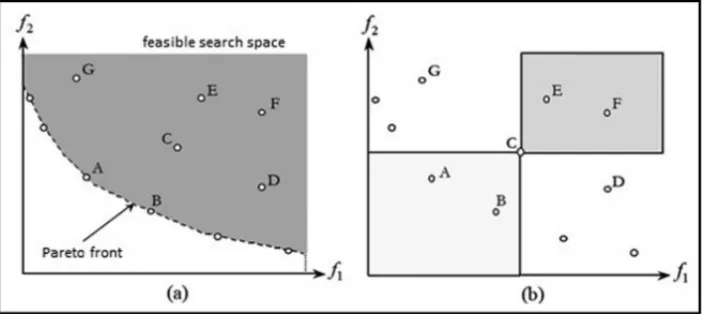
Figure 1 illustrates these ideas for a two-objective case. Solution C dominates E and F because their objective values for both f1and f2are greater than those for C. Meanwhile, the objective
values for A and B are smaller than those for solution C, and so both A and B dominate C. However neither G nor D dominate, or are dominated by, C.
Figure 1– Pareto dominance.
In the presence of multiple Pareto optimal solutions, it is not possible to prefer one solution over the other. In the absence of other information all Pareto optimal solutions are equally important, and in a typical real world situation the decision making process may take account of many factors which are time-dependent, subjective, or otherwise hard to quantify. Hence, heuristics for multi-objective optimization have two goals: 1) to find a set of solutions as close as possible to the Pareto front and 2) to find as diverse a set of solutions as possible. Taken to-gether this usually means that heuristics try to produce an approximation to the Pareto front in which solutions are sparsely spaced.
According to Fonseca & Fleming (1995), conventional optimization techniques, such as gradient-based and simplex-gradient-based methods are difficult to extend to the true multi-objective case, because they were not designed with multiple solutions in mind. In contrast to this, it has long been recognized that the population-based algorithms are potentially well-suited to multi-objective optimization.
Thus an Evolutionary Algorithm’s evolving population can search for multiple solutions in paral-lel, potentially exploiting similarities available in the family of possible solutions to the problem. So, the most striking difference to classical optimization algorithms is that EAs uses a population of solutions in each iteration instead of a single solution. If an optimization problem has a single optimum, then via genetic drift, all EA population members will converge to (an approximation of) that optimal solution. However, if an optimization problem has multiple optimal solutions, an EA can be used to approximate multiple optimal solutions in its final population; this ability to find multiple solutions makes EAs unique in solving multi-objective optimization problems (Deb, 2011).
The Vector Evaluated Genetic Algorithm (VEGA) sub-divide the population, using different ob-jectives to award fitness to different sub-populations (Schaffer, 1985). Goldberg (1989) suggested using the concept of domination, which was adopted and refined by many different implemen-tations of objective Optimization Evolutionary Algorithms (MOEAs), such as the Multi-objective Genetic Algorithm (MOGA) (Fonseca & Fleming, 1993), the Non-dominated Sorting Genetic Algorithm (NSGA) (Srinivas & Deb, 1994) and the Niched Pareto Genetic Algorithm (NPGA) (Horn et al., 1994). The literature on MOEA is now extensive and good surveys can be found in Chinchuluun & Pardalos (2007), Coello (2000), Ehrgott & Gandibleux (2000), Gong et al. (2009) and Zhou et al. (2011).
4.2 A Multi-objective Genetic Algorithm for the 1D-SSSCSP with Setups
In this study we propose a Genetic Algorithm (GA) to solve the bi-criteria problem which min-imizes both the waste of material and the number of different cutting patterns. The algorithm was adapted from Araujo et al. (2011) in order to deal with the two conflicting objective func-tions. Moreover, that paper considered minimizing the waste of material for the One Dimensional Multiple Stock Size Cutting Stock Problem (1D-MSSCSP) (W¨ascher et al., 2007) under the con-dition that production exactly met demand. In this paper we significantly extend the heuristic to tackle a multi-objective version of the One Dimensional Single Stock Size Cutting Stock Prob-lem (1D-SSSCSP) and we also allow inequalities – that is to say we allow for overproduction of items, with the excess quantities treated as waste.
We first discuss the way that fitness is assigned to a candidate solution in the context of the cur-rent population, then the selection processes via which individuals are selected for reproduction and survival. Next, we discuss the representation and the recombination operator that work on that representation to create new offspring, and finally the process via which the representation of a solution is transformed into a candidate solution.
Rank-based fitness assignment function: Fonseca & Fleming (1993) provide this non-dominated classification of a GA population. Consider an individual which is non-dominated byηi
individuals in the current population. It is given a rank τi = 1+ηi, so all non-dominated
The idea of using the ranking rather than raw fitness values to determine selection probabilities has been shown to combat premature convergence. In this case a simple linear ranking tech-nique is used to assign effective fitness. Ifµ(τi)denotes the number of solutions with rankτiin
population of total sizeP, then the fitness of any individual is given by:
Fi =P− τi−1
k=1
µ(k)−0,5(µ(τi)−1) i =1, . . . ,P. (6)
Equation (6) associates the same fitness for every solution of the same rank. To promote diver-sity among the non-dominated solutions, this fitness is then moderated to preferentially reward solutions that are dissimilar to others of the same rank. Letσsharebe a parameter that defines
how far apart two individuals must be in order for them to decrease each other’s fitness. The region within radiusσshareof a solution is called itsniche. For each solutioniand jof the same
rank, calculate the sharing function value which is given by:
Sh(di j)= ⎧ ⎨
⎩
1− d
i j
σshar e
β
, ifdi j ≤σshare
0, otherwise
(7)
whereβ is a parameter, typicallyβ ∈ [1,2], anddi j is the distance between the solutionsi and j. The distance metric used is the normalized Euclidean distance in objective function space:
di j =
q
k=1
fi k − f
j k fkmax− fkmin
2
(8)
whereq is the number of objectives, fkmaxand fkminare the maximum and minimum objective function value of thekth objective considering the current population, and fki is the objective function value of thekth objective of the solutioni.
We evaluate theniche countfor solutioni,nci as follows:
nci = µ(τi)
j=1
Sh(di j), i =1, . . . ,P. (9)
Then, we compute the shared fitness:
Fi′ = Fi nci
. (10)
Thus, when comparing two solutions of the same rank, the one from the less crowded region will have a higher shared fitness. Finally, to preserve the same average fitness for all solutions of the same rank and maintain selection pressure, we scale the shared fitness as per:
Fi′′= Fiµ(τi) µ(τi)
k=1 F
′
k
Parent selection: given the fitness scheme above we select individuals to be parents using fitness-proportionate selection, implemented via the “roulette wheel” algorithm. This is concep-tually the same as spinning a one-armed roulette wheel, where the sizes of the holes reflect the selection probabilities (Eiben & Smith, 2010).
Population replacement strategy: a steady-state model is used whereby one new individual is generated per iteration. If this is better than the worst individual of the current population, then the latter is eliminated and the new individual is included in the sorted population in the correct position.
Representation: consider an individual as a feasible solution for the cutting stock problem. The individual is made up of a number of genes, each of which represents a cutting pattern (aj) and also the number of times it is cut (xj). Therefore, an individual is represented as a
matrix where a column represents a cutting pattern (and the number of times it is cut). We allow individuals to contain different numbers of patterns, so the number of columns in the matrix representing an individual can be different, but the number of rows in each matrix is the same: equal to the number of different items (m) plus one row containing the number of times the cutting pattern is used.
Creation of initial population: in order to generate the initial population an adaptation of the simple Repeat Exhaustion Reduction (RER) Heuristic (Hinxman, 1980) is used. It can be summarized as follows.
Step 1:Construct a cutting patternaj.
Step 2:Apply this cutting pattern as many times as possible (i.e., determinexj), without
exceed-ing the demand for any item.
Step 3: Update the demand and repeat steps 1 and 2 until the demand is fully met (we have a feasible integer solution).
In order to assist evolutionary search the initial population should sample the search space, so it is important to generate individuals with different characteristics. Two different approaches were used to construct a cutting pattern in Step 1. Each of these ranks items in a different way and then selects items to go into the cutting pattern according to this rank:
RER 1: Rank items according to the First Fit Decreasing (FFD) heuristic (Johnson, 1974; W¨ascher & Gau, 1996).
Once a cutting pattern is constructed the number of times it will be cut, xj, is determined by
taking the maximum value possible, so that it does not overproduce the demand of any item that belongs to this cutting pattern.
One individual is constructed by using RER 1 and remaining individuals of the initial population are constructed using RER 2. The population-size is a parameter of the GA.
Offspring creation: to create a new individual firstly global recombination is applied to select up toggenes (cutting patterns), then, if necessary, a constructive heuristic is applied.
The recombination operator successively applies the selection operators described above to select a parent, and then chooses a random gene from that parent, taking care not to choose a gene which produces an item for which the residual demand has already been met. The parameterg
must be previously defined and it is based on the population characteristics. In this paper we use the mean number of cutting patterns of the individuals from the current population plus a certain percentage that gives a higher chance of selecting cutting patterns. If, beforegattempts, the demand for each item is met, then we have a feasible individual. Otherwise, an additional constructive heuristic phase is carried out in order to create a feasible solution. In this step, the Repeat Exhaustion Reduction heuristic (RER1) is used again, considering only the residual demand.
This differs from the traditional use of both recombination and a mutation operator to create necessary diversity to permit evolution. In our case diversity is created by (i) the use of heuris-tics to generate novel patterns continuously throughout the run, (ii) the use of randomized global recombination to select patterns into an offspring, coupled with (iii) the incorporation of con-structive heuristics within recombination to control how many patterns are added, and finally (iv) the use of the RER1 heuristic to create new patterns to meet residual demand if needed.
Definition of thexj-value: each time the recombination operator selects a gene, the associated
xj-value (number of times this cutting pattern will be repeated) is recalculated. Starting from
zero, we incrementally increasexj, noting the values at which the first and the last items have
their demand satisfied, and which those items are. We choosexj according to the value for the
last item if the overproduction of the first item is less than a parameter. Otherwise we choose
xj values which just meet demand for the first item. The parameteris related to the length of
overproduction.
The idea behind this procedure is that when we choosexj according to the last item, every item
that belongs to that cutting pattern will have its demand met, which should help reducing the number of cutting patterns needed, at the cost of some overproduction. Conversely, when we choosexj according to the first item, only this item will have its demand satisfied, consequently
Stopping criterion: it is defined as the maximum number of iterations, where each iteration represents the generation of an individual.
5 COMPUTATIONAL RESULTS
This section is divided in two parts. In the first one we used a set of forty “real-world” instances from the literature (Umetani et al., 2003), where results are available for several existing algo-rithms, giving the minimum loss solutions found for different (fixed) numbers of setups (cutting patterns). For each instance we compare these with the range of results found from a single run of the MOGA algorithm. We use a single run in these tests because the aim is to show the multi-objective aspects of the solutions. A statistical analysis will be done on the results presented in Section 5.2.
The second data set comprises 1800 instances generated by the Random Generator CUTGEN1 (Gau & W¨ascher, 1995). We compare the solution quality of our multi-objective approach against other single objective methods proposed in the literature. In this case we focus on the best solu-tion, in terms of number of objects to be cut, of our final population.
MOGA was implemented in C++ and the computational tests were carried out on an Intel(R) Core(TM) i5-2410M, CPU 2.30 GHz 2.30 GHz with 4.0 GB of RAM, under Windows 7 Professional.
Extensive computational tests were carried out and several parameters were tested. For the computational results, the parameters used in MOGA are: the size of the initial population was set equal to 50; the maximum number of genes (g) was based on the average of the number of genes of the individuals from the initial population plus 20%; the limit of overproduction () produced by a cutting pattern j when cut a number of times (xj) is fixed to 1.5L(see definition
of the xj-value in Section 4.2); the stopping criterion (maximum number of iterations) was set
to 5000 and the parameters related to the rank-based fitness function wasσshare = 2/(P−1)
andβ=1.
5.1 Practical Data Set
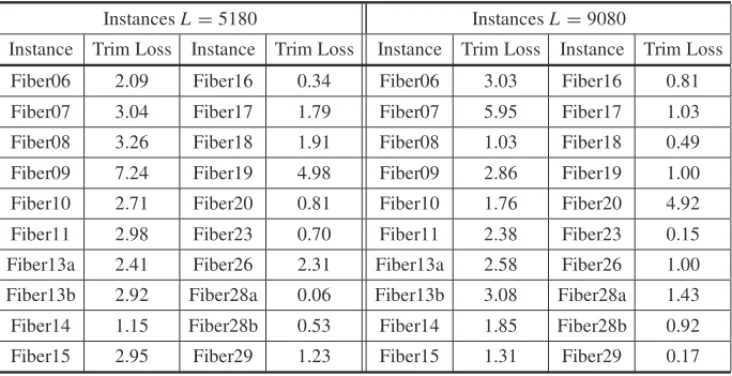
As in Lee (2007) and Golfeto et al. (2009b) we used the 40 instances available from Umetani et al. (2003). These instances come from a chemical fiber company in Japan:
• Number of types of ordered items:mvaries from 4 to 20;
• Object length: L = 5180 for the first 20 instances and L = 9080 for the remaining 20 instances;
• Item length:li were randomly generated in the interval[500,2000];
• Demand:bi were randomly generated in the interval[2,264]and we aggregated demand
bi of the items that have the same lengthli– which is common in the literature (Lee, 2007;
Table 1 shows the results, for each instance, of the optimal solution considering only the min-imization of the percentage of trim loss Eq. (5). These optimal solutions were found through the implementation of the arc flow model presented in Valerio de Carvalho (1999) and Valerio de Carvalho (2002) in the AMPL modeling language (Fourer et al., 2002) and solved with the optimizer CPLEX 12.1.
Table 1– Optimal solutions for trim loss Eq. (5) minimization.
InstancesL=5180 InstancesL=9080
Instance Trim Loss Instance Trim Loss Instance Trim Loss Instance Trim Loss
Fiber06 2.09 Fiber16 0.34 Fiber06 3.03 Fiber16 0.81
Fiber07 3.04 Fiber17 1.79 Fiber07 5.95 Fiber17 1.03
Fiber08 3.26 Fiber18 1.91 Fiber08 1.03 Fiber18 0.49
Fiber09 7.24 Fiber19 4.98 Fiber09 2.86 Fiber19 1.00
Fiber10 2.71 Fiber20 0.81 Fiber10 1.76 Fiber20 4.92
Fiber11 2.98 Fiber23 0.70 Fiber11 2.38 Fiber23 0.15
Fiber13a 2.41 Fiber26 2.31 Fiber13a 2.58 Fiber26 1.00
Fiber13b 2.92 Fiber28a 0.06 Fiber13b 3.08 Fiber28a 1.43
Fiber14 1.15 Fiber28b 0.53 Fiber14 1.85 Fiber28b 0.92
Fiber15 2.95 Fiber29 1.23 Fiber15 1.31 Fiber29 0.17
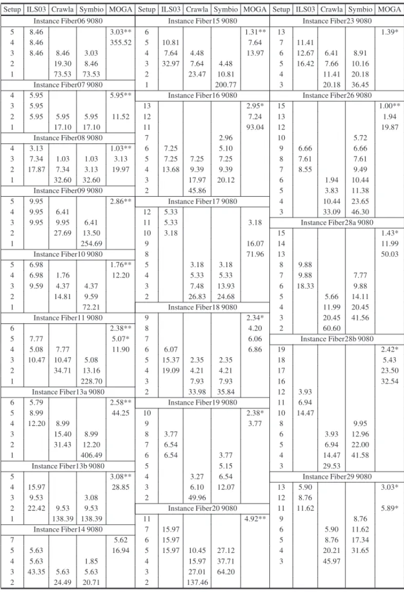
We compare the proposedMOGAmethod against three other methods from the literature that present sets of non-dominated solutions for these instances taken from multiple runs (in the case of the two local-search based methods):ILS03,CrawlaandSymbioproposed, respectively in Umetani et al. (2003), Lee (2007) and Golfeto et al. (2009b).
Tables 2 and 3 present the comparison of results for the instances where L = 5180 and
L = 9080, respectively. We present in the respective column of each method (ILS03, Crawla, Symbio, MOGA) the percentage of trim loss (evaluated according to Eq. (5)) obtained with the respective number of different cutting patterns (columns Setup).
Table 2– Setup and percentage trim loss obtained by the four methods (L=5180).
Setup ILS03 Crawla Symbio MOGA Setup ILS03 Crawla Symbio MOGA Setup ILS03 Crawla Symbio MOGA Instance Fiber06 5180 Instance Fiber14 5180 Instance Fiber23 5180
7 5.19 11 5.45 16 2.83*
6 5.19 2.09** 10 5.45 15 4.98 4.26
5 5.19 5.19 8.27 9 5.45 14 2.84
4 8.28 8.28 8 7.61 13 6.41
2 48.5 17.55 6 5.45 11 17.84 8.55
Instance Fiber07 5180 5 5.45 5.45 10 9.26
10 4.98 4 9.76 9.76 9 2.84 10.69
9 4.98 3 14.06 14.06 8 4.27 12.12
8 4.98 2 63.56 85.08 7 5.70 14.98
7 4.98 Instance Fiber15 5180 6 7.84 17.83
6 8.16 14 4.76 5 19.98 21.40
4 4.98 13 4.76 4 67.11
3 8.16 4.98 8.16 12 4.76 Instance Fiber26 5180
2 11.34 11.34 11 4.76 29 3.39
1 68.61 68.61 10 6.56 28 2.31
Instance Fiber08 5180 6 4.75* 27 3.39
10 4.47 5 8.36 26 3.39
9 4.47 4 4.76 4.76 11.81 25 3.93
8 4.47 3 10.17 6.56 14 3.93
7 4.47 2 49.91 39.07 13 5.00
6 4.47 Instance Fiber16 5180 12 10.39
5 3.26** 16 4.01 10 8.78
4 4.46 13 5.23 9 9.31
3 4.46 4.46 6.86 12 6.45 8 4.47 10.93
2 5.67 5.67 11 10.13 7 5.01 15.78
1 126.94 10 7.68 6 7.16
Instance Fiber09 5180 9 6.46 5 15.78 28.16
9 9.27 8 8.91 4 78.24 96.01
8 9.27 7 8.91 4.01 4.01 Instance Fiber28a 5180
7 11.29 9.26* 6 27.26 5.24 5.23 16 3.67*
6 11.29 5 11.35 7.68 14 4.87*
5 11.29 11.28 4 13.80 16.25 11 9.70
4 11.29 3 45.62 66.41 10 10.91 8.49
3 23.43 11.29 Instance Fiber17 5180 9 10.91 9.70 2 47.71 47.71 10 3.01* 8 18.14 4.88 13.31 Instance Fiber10 5180 9 5.46 5.30 7 26.58 7.29 19.34
14 4.20 8 6.69 4.24 9.63 6 9.70 32.60
13 4.20 7 7.92 44.52 5 13.32 50.69
12 4.20 6 17.28 4.24 5.46 4 28.99
11 4.20 5 22.63 6.69 6.69 Instance Fiber28b 5180
10 4.20 4 7.92 11.59 22 3.97*
6 4.20 3 29.99 29.99 18 4.83*
5 4.20 7.17 Instance Fiber18 5180 17 8.27 4 5.69 4.20 47.31 14 2.97* 15 5.69
3 7.18 5.69 12 4.03* 14 6.55 7.40
2 22.06 22.06 11 5.10 47.56 13 6.55 9.12
Instance Fiber11 5180 10 6.16 12 8.27
12 6.06 9 5.10 5.10 11 6.55 9.98
11 6.06 8 10.41 6.16 10 10.84
10 4.52 7 11.47 9 5.69 13.42
9 4.52 6 5.10 7.22 8 5.69 17.72
8 6.06 5 6.16 10.40 7 8.27 22.87
7 2.98** 4 7.22 11.46 6 15.14 41.78
6 9.13 3 18.90 82.59 5 34.90 96.77
5 6.06 12.20 Instance Fiber19 5180 Instance Fiber29 5180
4 7.59 6.65 14.67 25 4.98 22 2.86*
3 10.67 9.13 24 5.77 20 4.49*
2 52.16 23 4.98 19 7.76
Instance Fiber13a 5180 22 4.98 18 28.99
14 2.41 21 4.98 13 11.03
13 4.24 10 5.77 12 9.40
12 2.41 9 5.77 5.77 8.92 11 14.30 7.76
11 4.24 8 6.56 6.56 10 9.40 9.40
10 4.24 7 7.35 7.35 9 12.66 4.50 11.03
9 4.24 6 8.14 8.93 8 9.40 14.29
8 6.06 5 9.72 10.51 7 2.78 22.46
7 10.05 4 14.45 24.71 6 24.09 43.68
5 6.07 3 46.82 5 32.26 53.48
4 13.38 7.90 Instance Fiber20 5180
3 28.01 13.38 16 3.96*
2 51.79 15 7.11
Instance Fiber13b 5180 14 32.31
9 6.59 12 99.81
8 6.59 8 13.41
7 6.59 7 19.71 7.11 7.11
6 6.59 2.92** 6 26.02 10.26 13.41 5 6.59 10.26 5 54.37 22.86 16.56 4 6.59 6.59 4 57.52 54.37 3 10.27 10.27
Table 3– Setup and percentage trim loss obtained by the four methods (L =9080). Setup ILS03 Crawla Symbio MOGA Setup ILS03 Crawla Symbio MOGA Setup ILS03 Crawla Symbio MOGA
Instance Fiber06 9080 Instance Fiber15 9080 Instance Fiber23 9080
5 8.46 3.03** 6 1.31** 13 1.39*
4 8.46 355.52 5 10.81 7.64 7 11.41
3 8.46 8.46 3.03 4 7.64 4.48 13.97 6 12.67 6.41 8.91
2 19.30 8.46 3 32.97 7.64 4.48 5 16.42 7.66 10.16
1 73.53 73.53 2 23.47 10.81 4 11.41 20.18
Instance Fiber07 9080 1 200.77 3 20.18 36.45
4 5.95 5.95** Instance Fiber16 9080 Instance Fiber26 9080
3 5.95 13 2.95* 15 1.00**
2 5.95 5.95 5.95 11.52 12 7.24 13 1.94
1 17.10 17.10 11 93.04 12 19.87
Instance Fiber08 9080 7 2.96 10 5.72
4 3.13 1.03** 6 7.25 5.10 9 6.66 6.66
3 7.34 1.03 1.03 3.13 5 7.25 7.25 7.25 8 7.61 7.61
2 17.87 7.34 3.13 19.97 4 13.68 9.39 9.39 7 8.55 9.49
1 32.60 32.60 3 17.97 20.12 6 1.94 10.44
Instance Fiber09 9080 2 45.86 5 3.83 11.38
5 9.95 2.86** Instance Fiber17 9080 4 10.44 23.65
4 9.95 6.41 12 5.33 3 33.09 46.30
3 9.95 9.95 6.41 11 5.33 3.18 Instance Fiber28a 9080
2 27.69 13.50 10 3.18 15 1.43*
1 254.69 9 16.07 14 11.99
Instance Fiber10 9080 8 71.96 13 50.03
5 6.98 1.76** 5 3.18 3.18 8 9.88
4 6.98 1.76 12.20 4 5.33 5.33 7 9.88 7.77
3 9.59 4.37 4.37 3 7.48 13.93 6 18.33 9.88
2 14.81 9.59 2 26.83 24.68 5 5.66 14.11
1 72.21 Instance Fiber18 9080 4 11.99 20.45
Instance Fiber11 9080 9 2.34* 3 20.45 41.56
6 2.38** 8 4.20 2 60.60
5 7.77 5.07* 7 6.06 Instance Fiber28b 9080
4 5.08 7.77 11.90 6 6.07 6.86 19 2.42*
3 10.47 10.47 5.08 5 15.37 2.35 2.35 18 5.43
2 34.71 13.16 4 19.09 4.21 4.21 17 23.50
1 228.70 3 7.93 7.93 16 32.54
Instance Fiber13a 9080 2 33.98 35.84 12 3.93
6 5.79 2.58** Instance Fiber19 9080 11 6.94
5 8.99 44.25 10 2.38* 10 14.47
4 12.20 8.99 9 3.77 8 9.95
3 15.40 8.99 8 3.77 6 3.93 12.96
2 31.43 12.20 7 6.54 5 6.94 22.00
1 406.49 6 6.54 3.77 4 14.47 41.58
Instance Fiber13b 9080 5 5.15 3 29.53
5 3.08** 4 3.27 6.54 Instance Fiber29 9080
4 15.97 28.85 3 6.10 12.07 13 5.90 3.03*
3 9.53 3.08 2 49.96 12 8.76
2 22.42 9.53 9.53 Instance Fiber20 9080 11 11.62 5.89*
1 138.39 138.39 11 4.92** 9 8.76
Instance Fiber14 9080 7 15.97 6 5.90 11.62
7 5.62 6 15.97 5 8.76 17.34
5 5.63 16.94 5 15.97 10.45 27.12 4 20.21 31.65
4 5.63 1.85 4 15.97 37.71 3 45.97
3 43.35 5.63 5.63 3 27.01 64.20
Comparing our results with the results from Golfeto et al. (2009b), we can see that we obtained complementary results, i.e., we found solution with less trim losses and more setups, which confirms the difference between these two solution methods. It is possible to see that for some instances they are far from the optimal trim loss. Our complementary results can be important depending on the characteristics of the (practical) problem we are solving. Another point that must be highlighted is that our method is quite efficient, and it takes on average around 5 seconds to solve each instance, while their method took between 60 and 80 minutes for solving each instance. So, it is possible to conclude that the proposed multi-objective GA appears as a very simple and efficient alternative for producing non-dominated solutions for these 40 practical instances.
5.2 Randomly Generated Data Set
The eighteen classes of instances generated by the Random Generator CUTGEN1 (Gau & W¨ascher, 1995) were used. For each class, 100 instances were generated and solved. So, the 1800 instances were generated according to the following parameters (Table 4):
• Number of types of ordered items:m=10,20 and 40;
• Object length:L =1000;
• Item length: li were randomly generated in the interval[v1L, v2L]; with lower bound
v1=0.01 and 0.2, and upper boundv2=0.2 and 0.8;
• Average demand (b¯) (bi,i =1, . . . ,m): 10 and 100.
For each class, the fifth column of Table 4 also shows the mean of the optimal solution for the number of objects nj=1xj, considering the single objective problem of minimizing the
number of objects. The sixth column shows the lower bounds for number of different cutting patternsnj=1δ(xj). The optimal solutions were obtained as in Table 1 and the lower bounds
were presented in Yanasse & Limeira (2006).
In Table 5 we present the computational results comparing our MOGA, using the same param-eters as above, with the results from four previously published methods. For each presented method, the first column is the number of objects, nj=1xj, and the second column is the
number of different cutting patterns, nj=1δ(xj). These four methods are: KOMBI, HH, ILS06andSymbio1proposed, respectively, in Foerster & W¨ascher (2000), Yanasse & Limeira (2006), Umetani et al. (2006) and Golfeto et al. (2009a). We considered Symbio1 because this method presented the best results in terms of number of objects when compared to Symbio5 and Symbio10.
Table 4– Parameters for the random instances, optimal solution and bounds.
Class b m v1andv2
Optimal solution Lower bounds n
j=1xj nj=1δ(xj)
C1 10 10 0.01 and 0.2 11.48 1.66
C2 100 10 0.01 and 0.2 110.25 1.66
C3 10 20 0.01 and 0.2 22.13 2.55
C4 100 20 0.01 and 0.2 215.93 2.55
C5 10 40 0.01 and 0.2 42.95 4.25
C6 100 40 0.01 and 0.2 424.68 4.25
C7 10 10 0.01 and 0.8 50.24 4.99
C8 100 10 0.01 and 0.8 499.62 4.99
C9 10 20 0.01 and 0.8 93.81 9.24
C10 100 20 0.01 and 0.8 932.26 9.24
C11 10 40 0.01 and 0.8 176.9 16.92
C12 100 40 0.01 and 0.8 1763.45 16.92
C13 10 10 0.2 and 0.8 63.47 6.27
C14 100 10 0.2 and 0.8 632.36 6.27
C15 10 20 0.2 and 0.8 119.59 11.76
C16 100 20 0.2 and 0.8 1192 11.76
C17 10 40 0.2 and 0.8 222.76 21.98
C18 100 40 0.2 and 0.8 2221.56 21.98
methods, the results for the MOGA present the non-dominated solution of the final population with the fewest objects. Observe that we could choose another non-dominated solution. To give an idea of the number of non-dominated solutions, we include two additional columns for the MOGA. Column ND is the average number of non-dominated solutions. These solutions have different cutting patterns and/or different frequencies. However, some of these solutions have the same value for the number of cut objects nj=1xj and for the number different cutting
patternsnj=1δ(xj). So, DND is the average number of non-dominated solutions with different
values for the number of cut objectsnj=1xj and/or for the number different cutting patterns n
j=1δ(xj).
A G EN ET IC AL G O R IT H M F O R T H E O N E-D IM E N S IO N A L C U T T IN G ST O C K P R O BL EM WI T H SET U P S
KOMBI HH ILS06 Symbio1 MOGA
Class n
j=1
xj n
j=1 δ(xj)
n
j=1
xj
n
j=1 δ(xj)
n
j=1
xj
n
j=1 δ(xj)
n
j=1
xj n
j=1 δ(xj)
n
j=1
xj n
j=1
δ(xj) ND* DND*
1 11.49 3.40 11.56 3.31 12.24 2.43 12.59 3.09 11.59 6.46 35.85 2.31
2 110.25 7.81 110.4 6.95 114.49 3.18 115.17 6.11 111.25 13.51 6.08 3.04
3 22.13 5.89 22.17 4.96 23.53 3.98 25.96 5.74 23.30 15.73 6.84 2.31
4 215.93 14.26 215.98 10.32 223.92 4.89 235.93 10.59 217.71 29.47 5.38 5.30
5 42.96 10.75 42.99 7.63 45.29 6.68 57.17 9.89 45.29 33.00 4.12 4.00
6 424.71 25.44 424.89 13.31 442.00 7.25 472.95 30.07 426.98 62.38 8.17 8.17
Avg. 137.91 11.26 138 7.75 143.58 4.73 153.29 10.91 139.35 26.76 11.07 4.18
7 50.21 7.9 51.69 7.66 51.35 5.52 51.58 6.36 54.56 8.98 29.63 2.04
8 499.52 9.96 502.23 9.62 507.92 5.75 510.5 8.51 501.16 10.91 20.52 2.3
9 93.67 15.03 99.49 13.64 96.35 10.05 99.36 10.94 98.94 19.33 5.55 3.04
10 932.32 19.28 948.41 18.21 954.55 10.30 970.57 16.7 936.84 22.85 5.01 3.53 11 176.97 28.74 195.67 24.6 182.88 18.32 198.26 23.04 186.90 39.59 4.25 4.17
12 1766.20 37.31 1847.42 33.23 1818.35 18.40 1932.16 32.93 1771.97 44.77 4.01 3.99
Avg. 586.48 19.7 607.48 17.82 601.9 11.39 627.07 16.41 591.73 24.41 11.49 3.17
13 63.27 8.97 64.20 8.93 64.16 6.68 65.23 7.28 81.25 9.57 31.62 1.85
14 632.12 10.32 633.26 10.51 637.03 6.85 646.77 8.62 633.48 10.53 29.76 1.8 15 119.43 16.88 123.9 16.28 122.44 12.34 127.39 13.66 126.20 19.09 12.5 2.6
16 1191.80 19.91 1197.66 19.89 1217.91 12.46 1254.69 16.68 1195.92 21.26 11.02 2.69 17 224.68 31.46 244.02 29.76 231.41 22.44 244.49 27.22 237.25 39.18 4.27 4.18
18 2242.4 38.28 2268.3 37.9 2307.70 22.50 2414.07 32.7 2249.79 41.88 3.71 3.69
Avg. 745.67 20.97 755.22 20.54 763.44 13.88 792.10 17.69 753.98 23.58 15.48 2.80
*ND is the average number of non-dominated solutions and DND is the average number of different non-dominated
solutions, i.e., solutions with different values for the number of cut objectsn x and/or for the number different
We can conclude that, taking the best solution in terms of number of objects, our method pro-duces good results when the number of objects is analyzed, but this solution is not good in terms of the number of different cutting patterns. However, the reader should be aware that this com-parison only considers the member of final population with the fewest objects – and that since the algorithm is designed to produce a diverse set of solutions, others will have different trade-offs between objects and cutting patterns. On overall average our method produced 3.4 different non-dominated solutions for each instance. Since the number of cutting patterns is integer this limits the possible diversity and 3.4 seems to be a good number of non-dominated solutions. Considering the computational time, it is not easy to do a complete comparison because of the difference between the machines. However, it is possible to observe in Table 6 that our method is relatively fast (it takes, on average, 11.48 seconds to solve each instance). Moreover, it is relatively robust and does not vary much according to the characteristics of the instances (see, for instance, class C12).
Table 6– Average CPU time (in seconds) for each method.
Class KOMBI HH ILS06 Symbio5 MOGA
C1 0.14 0.23 0.10 18.54 3.55
C2 1.14 0.48 0.22 37.88 5.02
C3 1.74 0.12 0.72 33.25 5.17
C4 16.00 2.75 2.69 68.11 6.21
C5 38.03 3.43 7.55 58.29 18.12
C6 379.17 7.81 23.18 158.04 28.95
C7 0.07 0.11 0.21 19.62 14.77
C8 0.20 0.60 0.27 48.48 8.46
C9 3.37 0.49 1.96 38.75 6.46
C10 3.25 3.36 2.19 127.25 5.40
C11 36.26 7.17 19.16 117.85 29.14
C12 76.31 44.62 23.87 426.08 27.16
C13 0.08 0.13 0.26 17.66 7.82
C14 0.13 0.25 0.31 31.19 10.10
C15 1.81 0.97 2.01 41.12 6.19
C16 2.60 2.46 2.21 133.90 4.42
C17 50.93 15.46 22.01 153.45 10.36
C18 70.94 50.61 26.84 388.89 9.26
Average 37.90 7.84 7.54 106.58 11.48
Note: CPU time for KOMBI234 was on a 486/66 processor, for ILS06
was on a Pentium IV (2 GHz) processor, for HH was on a Intel Celeron
(266 MHz) processor and for Symbio5 was on a AMD SEMPRON
Regarding the direct comparison between the two GAs, observe that in Tables 5 and 6 we com-pare our method, which finds, for each instance, a set of non-dominated solutions, against other methods including the method presented in Golfeto et al. (2009a) which finds only one solution for each instance. Referring to the results presented in Table 5, we are comparing our method against Symbio1 which is the best (in terms of saving in waste) single objective method pre-sented in Golfeto et al. (2009a). Even comparing with Symbio1, we obtain slightly better results. A comparison with Symbio5 or Symbio10 would give a more explicit difference in favor of our method. Moreover, Table 6 shows that, on average, our method took only 11.47 seconds, while their method took 106.58 seconds to solve each instance. It is worth re-emphasizing that our method finds a set of non-dominated solution while their method finds only one solution.
6 CONCLUSION AND FUTURE RESEARCH
This paper dealt with the one-dimensional cutting stock problem considering two conflicting objectives. In practice, hundreds of different items may need to be cut, requiring thousands of different cutting patterns, which makes even the minimization of loss problem difficult to solve. When other practical aspects, such as reducing production time lost to set-ups are taken into account, the resulting nonconvex multi-objective function is far more complex. In order to deal with this difficulty, we have proposed a straightforward multi-objective genetic algorithm. The proposed method is very simple, flexible in terms of the objective function to be minimized and relatively efficient in terms of computational time. Considering the quality of the produced solution, the method is competitive with other methods from the literature and it has the advan-tage of producing a set of non-dominated solutions, from which the decision maker can choose according to the many factors which influence businesses.
ACKNOWLEDGMENTS
The authors would like to thank the Brazilian agencies CAPES, CNPq, FAPESP (Process 2011/ 22647-0) and the European Union (Project 2012/00464-4) for financial support.
REFERENCES
[1] ALVESC, MACEDOR & VALERIO DECARVALHOJM. 2009. New lower bounds based on column generation and constraint programming for the pattern minimization problem.Computers & Opera-tions Research,36(11): 2944–2954.
[2] ALVESC & VALERIO DECARVALHOJM. 2008. A branch-and-price-and-cut algorithm for the pat-tern minimization problem.RAIRO Operations Research,42(4): 435–453.
[3] ARAUJO SA, CONSTANTINO AA & POLDI KC. 2011. An evolutionary algorithm for the one-dimensional cutting stock problem. International Transactions in Operational Research, 18(1): 115–127.
[5] CERQUEIRAG & YANASSEH. 2009. A pattern reduction procedure in a one-dimensional cutting stock problem by grouping items according to their demands.Journal of Computational Interdisci-plinary Sciences,1(2): 159–64.
[6] CHINCHULUUNA & PARDALOSP. 2007. A survey of recent developments in multiobjective opti-mization.Annals of Operations Research,154(1): 29–50.
[7] COELLO CAC. 2000. An updated survey of GA-based multi-objective optimization techniques. ACM Computing Surveys,32(2): 109–143.
[8] CUIY & LIUZ. 2011. C-sets-based sequential heuristic procedure for the one-dimensional cutting stock problem with pattern reduction.Optimization Methods and Software,26(1): 155–67.
[9] DEBK. 2011.Multi-objective optimization using evolutionary algorithms. John Wiley & Sons Ltd, United Kingdom.
[10] DIEGELA, CHETTYM, VANSCHALKWYKS & NAIDOOS. 1993. Setup combining in the trim loss problem—3to2 & 2to1. Working paper. Business Administration. University of Natal. Durban. First Draft.
[11] DYCKHOFFH, SCHEITHAUERG & TERNOJ. 1997. Cutting and packing. In:Annoted Bibliogra-phies in Combinatorial Optimization[edited by DELL’AMICO M, MAFFIOLIF & MARTELLOS], John Wiley & Sons, Chichester, 393–413.
[12] EHRGOTTM. 2005.Multicriteria optimization. Springer Verlag, Berlin.
[13] EHRGOTT M & GANDIBLEUXX. 2000. A survey and annotated bibliography of multiobjective combinatorial optimization.OR Spektrum,22(4): 425–460.
[14] EIBENAE & SMITHJ. 2010.Introduction to evolutionary computing. Natural computating series. Springer-Verlag, Berlin Heidelberg.
[15] FARLEY AA & RICHARDSON KV. 1984. Fixed charge problems with identical fixed charges. European Journal of Operational Research,18(2): 245–249.
[16] FOERSTERH & W ¨ASCHERG. 2000. Pattern reduction in one-dimensional cutting stock problem. International Journal of Production Research,38(7): 1657–1676.
[17] FOGELDB. 2005.Evolutionary computation: Toward a New Philosophy of Machine Intelligence. IEEE Press Series on Computational Intelligence. John Wiley & Sons, USA.
[18] FONSECACM & FLEMINGPJ. 1993. Genetic algorithms for multiobjective optimization: formula-tion, discussion and generalization. In:Proceedings of the Fifth International Conference on Genetic Algorithms[edited by FORRESTS], Morgan Kaufmann Publishers Inc, 416–423.
[19] FONSECACM & FLEMINGPJ. 1995. An overview of evolutionary algorithms in multiobjective optimization.Evolutionary Computation,3(1): 1–16.
[20] FOURERR, GAYDM & KERNIGHANBW. 2002.AMPL: A modeling language for mathematical programming. Duxbury Press, Belmont.
[21] GAUT & W ¨ASCHERG. 1995. CUTGEN1: A problem generator for the one-dimensional cutting stock problem.European Journal of Operational Research,84(3): 572–579.
[23] GOLFETORR, MORETTIAC & SALLESNETOLL. 2009a. A genetic symbiotic algorithm applied to the one-dimensional cutting stock problem.Pesquisa Operacional,29(2): 365–382.
[24] GOLFETORR, MORETTIAC & SALLESNETOLL. 2009b. A genetic symbiotic algorithm applied to the cutting stock problem with multiple objectives.Advanced Modeling and Optimization,11(4): 473–501.
[25] GONGM, JIAOL, YANGD & MAW. 2009. Research on evolutionary multi-objective optimization algorithms.Journal of Software,20(2): 271–289.
[26] HAESSLER RW. 1975. Controlling cutting pattern changes in one-dimensional trim problems. Operations Research,23(3): 483–493.
[27] HAESSLERRW & SWEENEYPE. 1991. Cutting stock problem and solution procedures.European Journal of Operational Research,54(2): 141–150.
[28] HENN S & W ¨ASCHER G. 2013. Extensions of cutting problems: setups.Pesquisa Operacional, 33(3): 133–162.
[29] HERTZ A & KOBLERD. 2000. A framework for the description of evolutionary algorithms. Euro-pean Journal of Operation Research,126(1): 1–12.
[30] HINXMANA. 1980. The trim-loss and assortment problems: a survey.European Journal of Opera-tional Research,5(1): 8–18.
[31] HORN J, NAFPLIOTISN & GOLDBERGDE. 1994. A niched Pareto genetic algorithm for multi-objective optimization. In:Proceedings of the First IEEE Conference on Evolutionary Computation, IEEE World Congress on Computational Intelligence[edited by FOGELDD], IEEE,1: 82–87. [32] JOHNSONDS. 1974. Fast algorithms for bin packing.Journal of Computer and System Sciences,
8(3): 272–314.
[33] KOLENAWJ & SPIEKSMAFCR. 2000. Solving a bi-criterion cutting stock problem with open-ended demand: a case study.Journal of the Operational Research Society,51(11): 1238–1247.
[34] LEE J. 2007. In situ column generation for a cutting-stock problem. Computers & Operations Research,34(8): 2345–2358.
[35] MCDIARMIDC. 1999. Pattern minimisation in cutting stock problems.Discrete Applied Mathemat-ics,98(1-2): 121–130.
[36] MICHALEWICZZ. 1994.Genetic Algorithms+Data Structures=Evolution Programs. Springer-Verlag, New York.
[37] MOBASHERA & EKICIA. 2013. Solution approaches for the cutting stock problem with setup cost. Computers & Operations Research,40(1): 225–35.
[38] MORABITOR, ARENALESMN & YANASSEHH. 2009. Special issue on cutting, packing and related problems.International Transactions in Operations Research,16(6).
[39] MORETTIAC & SALLESNETOLL. 2008. Nonlinear cutting stock problem model to minimize the number of different patterns and objects.Computational and Applied Mathematics,27: 61–78. [40] OLIVEIRA JF & W ¨ASCHERG. 2007. Cutting and packing.European Journal of Operational
Re-search,183(3): 1106–1108.
[42] POLDIKC & ARENALESMN. 2010. O problema de corte de estoque unidimensional multiper´ıodo. Pesquisa Operacional,30: 153–174.
[43] SCHAFFERJD. 1985. Multiple objective optimization with vector evaluated genetic algorithms. In: Proceedings of the First International Conference on Genetic Algorithms[edited by GREFENSTETTE JJ], Lawrence Erlbaum Associates, 93–100.
[44] SRINIVASN & DEBK. 1994. Multi-objective function optimization using non-dominated sorting genetic algorithms.Evolutionary Computation Journal,2(3): 221–248.
[45] STEUERRE. 1985.Multiple criteria optimization: Theory, computation and application. John Wiley & Sons, New York.
[46] UMETANIS, YAGIURAM & IBARAKIT. 2003. An LP-based local search to the one dimensional cutting stock problem using a given number of cutting patterns.IEICE Transactions on Fundamentals of Electronics, Communications and Computer Sciences, E86-A, 1093–1102.
[47] UMETANIS, YAGIURAM & IBARAKIT. 2006. One dimensional cutting stock problem with a given number of setups: A hybrid approach of metaheuristics and linear programming.Journal of Mathematical Modelling and Algorithms,5(1): 43–64.
[48] VALERIO DECARVALHOJM. 1999. Exact solution of bin-packing problems using column genera-tion and branch-and-bound.Annals of Operations Research,86: 629–659.
[49] VALERIO DECARVALHOJM. 2002. LP models for bin packing and cutting stock problems. Euro-pean Journal of Operational Research,141(2): 253–273.
[50] VANVELDHUIZENDA & LAMONTGB. 2000. Multiobjective evolutionary algorithms: analyzing the state-of-the-art.Evolutionary Computation,8(2): 125–147.
[51] VANDERBECKF. 2000. Exact algorithm for minimizing the number of setups in the one-dimensional cutting stock problem.Operations Research,48(6): 915–926.
[52] WANGPY & W ¨ASCHER G. 2002. Editorial on cutting and packing.European Journal of Opera-tional Research,141(2): 239–240.
[53] W ¨ASCHERG & GAUT. 1996. Heuristics for the integer one-dimensional cutting stock problem: A computational study.OR Spektrum,18(3): 131–144.
[54] W ¨ASCHERG, HAUSSNERH & SCHUMANNH. 2007. An improved typology of cutting and packing problems.European Journal of Operational Research,183(3): 1109–1130.
[55] YANASSEHH & LIMEIRAMS. 2006. A hybrid heuristic to reduce the number of different patterns in cutting stock problems.Computers & Operations Research,33(9): 2744–2756.