❊♥s❛✐♦s ❊❝♦♥ô♠✐❝♦s
❊s❝♦❧❛ ❞❡
Pós✲●r❛❞✉❛çã♦
❡♠ ❊❝♦♥♦♠✐❛
❞❛ ❋✉♥❞❛çã♦
●❡t✉❧✐♦ ❱❛r❣❛s
◆◦ ✸✷✸ ■❙❙◆ ✵✶✵✹✲✽✾✶✵
❚❤❡ ❊✛❡❝t ♦❢ ■♥✢❛t✐♦♥ ♦♥ ●r♦✇t❤ ■♥✈❡st✲
♠❡♥ts✿ ❆ ◆♦t❡
❈❧♦✈✐s ❞❡ ❋❛r♦
❆❜r✐❧ ❞❡ ✶✾✾✽
❖s ❛rt✐❣♦s ♣✉❜❧✐❝❛❞♦s sã♦ ❞❡ ✐♥t❡✐r❛ r❡s♣♦♥s❛❜✐❧✐❞❛❞❡ ❞❡ s❡✉s ❛✉t♦r❡s✳ ❆s
♦♣✐♥✐õ❡s ♥❡❧❡s ❡♠✐t✐❞❛s ♥ã♦ ❡①♣r✐♠❡♠✱ ♥❡❝❡ss❛r✐❛♠❡♥t❡✱ ♦ ♣♦♥t♦ ❞❡ ✈✐st❛ ❞❛
❋✉♥❞❛çã♦ ●❡t✉❧✐♦ ❱❛r❣❛s✳
❊❙❈❖▲❆ ❉❊ PÓ❙✲●❘❆❉❯❆➬➹❖ ❊▼ ❊❈❖◆❖▼■❆ ❉✐r❡t♦r ●❡r❛❧✿ ❘❡♥❛t♦ ❋r❛❣❡❧❧✐ ❈❛r❞♦s♦
❉✐r❡t♦r ❞❡ ❊♥s✐♥♦✿ ▲✉✐s ❍❡♥r✐q✉❡ ❇❡rt♦❧✐♥♦ ❇r❛✐❞♦ ❉✐r❡t♦r ❞❡ P❡sq✉✐s❛✿ ❏♦ã♦ ❱✐❝t♦r ■ss❧❡r
❉✐r❡t♦r ❞❡ P✉❜❧✐❝❛çõ❡s ❈✐❡♥tí✜❝❛s✿ ❘✐❝❛r❞♦ ❞❡ ❖❧✐✈❡✐r❛ ❈❛✈❛❧❝❛♥t✐
❞❡ ❋❛r♦✱ ❈❧♦✈✐s
❚❤❡ ❊❢❢❡❝t ♦❢ ■♥❢❧❛t✐♦♥ ♦♥ ●r♦✇t❤ ■♥✈❡st♠❡♥ts✿ ❆ ◆♦t❡✴ ❈❧♦✈✐s ❞❡ ❋❛r♦ ✕ ❘✐♦ ❞❡ ❏❛♥❡✐r♦ ✿ ❋●❱✱❊P●❊✱ ✷✵✶✵
✭❊♥s❛✐♦s ❊❝♦♥ô♠✐❝♦s❀ ✸✷✸✮
■♥❝❧✉✐ ❜✐❜❧✐♦❣r❛❢✐❛✳
INVESTMENTS : A NOTE
CLOVIS DE FARO
1Revised
May, 1998
1
THE EFFECT OF INFLATION ON GROWTH
INVESTMENTS: A NOTE
I. Introduction
One of the most traditional issues in the theory of capital, is the choice of the optimal duration of growth investments. This problem, also known as capital deepening (cf. Baumol, 1972 and Hirshleifer, 1970) and which can be traced back to the 19th century work of the English mathematician W.S. Jevons, is typical of the so called point-input, point-output process. Illustrated, in an idealized way, by the activities of wine aging and tree growing, it consists of determining the length of time that an investor should keep an asset whose value increases with time.
Although a standard topic in text-books presentation of capital theory (besides the above mentioned works of Baumol and Hirshleifer, see, for instance: Allen, 1938; Bierman and Smidt, 1993; Henderson and Quandt, 1971; Simon and Blume, 1994 and Varian, 1990), the effects of inflation and taxation are usually not included in the analysis. Brenner and Venezia (1983) appear to be the first authors to take into account the joint effect of taxes and inflation on the optimal duration. However, despite the importance of their analysis, the very fact of considering the joint effect of taxes and inflation rendered some of the results somewhat confusing.
A previous note focused attention on the isolated effect of taxation on the optimal duration in a non-inflationary environment (de Faro, 1996). Complementing the analysis, the present note is aimed at the investigation of the effects of inflation by itself. Specifically, considering the no-reinvestment case only, our objective is to include in the analysis both a numerical illustration of the peculiar results of BV as well as some indexation procedures that have been used in some high inflation economies.
II. Basic Model
Adapting the notation in BV, let
f(T) - pre tax net receipt, as measured in monetary units referred to the date of the investment, derived from termination at time T;
h(T) - pre tax net receipt, as measured in nominal terms, derived from termination at time T; R - real rate of interest (as measured in instantaneous terms and assumed to be positive); C - cost of investment, as measured in monetary units referred to the date of the investment; T - time to termination of investment;
θ - constant rate of inflation (as measured in instantaneous terms and assumed to be positive);
ϕ - tax rate.
Assuming that the asset can be depreciated, for tax purposes, in a lump sum at the time of termination, with no indexation of the investment cost, and that the pre tax net receipt is fully indexed
(i.e. h(T) = eθΤf (T)), the cash flow associated with the investment, as expressed in current prices (i.e. nominal terms), is as depicted in Figure I
eθT
f T
( )
−
ϕ
(
e
θTf T
( )
−
C
)
0
T time
C
Figure I
Cash-Flow for the Basic Model
The above cash-flow corresponds to what will be called the basic model, and is the one that was addressed by BV.
Working with constant prices, as referred to the date of the investment, it follows that the function whose maximization determines the optimal duration is:1
F(T)= - C + e−( +θ)T
{
(
−
ϕ
)
θT( )
T
+
ϕ
C
}
f
e
1
R
(1)
1
3
Repeating here, for completeness, the presentation of BV, we have:
(
) ( )
(
( )
)
(
)
{
}
( )dF T
dT f T Rf T e R C e
T R T
( )
= − ′ − − + − +
1 ϕ θ θ ϕ θ (2)
Thus
( )
(
)
(
( )
( )
)
(
)
dF T
dT f T Rf T e R
T
= ⇒0 1−ϕ ′ − θ − +θ ϕC=0 (3)
On the other hand
( ) ( ) ( )
{
(
( )
)
(
) ( )
(
( )
)
}
( )d F T
dT
f
T
Rf
T e
f
T
Rf T e
e
T T R T
2
2
=
1
−
′′
−
′
+
1
−
′
−
− +
ϕ
θθ
ϕ
θ θ(
) ( )
− +
R
dF T
dT
θ
(4)Therefore, denoting by T* the solution of (3), we have:
( )
(
) ( )
{
( )
(
( )
( )
)
}
d F T
dT
Tf
T
Rf
T
f
T
Rf T
e
RT 2 2
1
= −
′′
−
′
+
′
−
− **
*
*
*
*ϕ
θ
(5)Thus, as 1-ϕ>0 and e−RT >0, it follows that T* will be the optimal duration if
( )
( )
(
( )
( )
)
′′ − ′ + ′ − <
f T* Rf T* θ f T* Rf T* 0 (6)
(
) ( )
(
( )
)
(
) ( )
{
( )
(
( )
( )
)
}
dT
d
C
T
f
T
Rf T e
f
T
Rf
T
f
T
Rf T
e
T T
θ
ϕ
ϕ
ϕ
θ
θ θ=
−
−
′
−
−
′′
−
′
+
′
−
1
1
(7)Taking into account (6), we know that, at T*, the denominator of (7) is negative. Accordingly, the sign of dT* / dθ is the opposite of the sign of the numerator of (7), which depends on T*.
Rather than pursuing the examination of the sign of the numerator of (7), a cumbersome task
indeed, BV turned their attention to the investigation of the sign of ∂ 2F(T) / (∂T ∂θ), at T*, as it is the same as the sign of dT/dθ, also at T*.1
From (2), it follows that
( )
{
(
) ( )
(
( )
)
}
( )∂
∂ ∂θ
ϕ
ϕ
θ θ
2
1
F T
T
T
f
T
Rf T e
C e
T R T
=
−
′
−
−
− +-T
{
(
1
−
ϕ
) ( )
(
f
′
T
−
Rf T e
( )
)
θT−
(
R
+
θ ϕ
)
C e
}
− +(R θ)TThus, taking into account (3), we have:
.
( )
{
*
(
) ( )
(
*
( )
*
)
}
( )*
* *
∂
∂ ∂θ
ϕ
θϕ
θ
2
1
F T
T
TT
f
T
Rf T
e
C e
T R T
=
−
′
−
−
− +or, given that
(
1−ϕ) ( )
(
f ′ T* −Rf T( )
*)
e−θT* =(
R+θ ϕ)
C( )
{
(
)
}
( )∂
∂ ∂θ
θ ϕ
ϕ
θ
2
F T
T
TT
R
C
C e
R T
=
+
−
− + * **
=
ϕ
C T
{
*
(
R
+ −
θ
)
1
}
e
− +(R θ)T* (8)
1
5
Therefore, the sign of dT/dθ at T* is the same as the sign of T* (R+θ) - 1. Thus, as R+θ was assumed to be positive, it follows that:
dT d
*
θ >
<0 if T* > < +
1
R θ (9)
or
dT d
*
θ >
<0 if θ >< −
1
T* R (10)
Quoting BV, we can say that “for investments with long duration increased inflation increases duration and the opposite holds for short duration. Alternatively, as expressed by (10), at high levels of inflation, increased inflation calls for longer duration and the opposite holds at low levels of inflation. In particular, a change from no inflation to some low level of inflation should decrease optimal duration”.
With the sole purpose to give at least some evidence of the magnitude of the numerical results that may be obtained, let us consider the case where, following an adaptation of an example that was presented in Hirshleifer (1970, pg, 87), we have :
f (T) = 90 log (1 + T) + 120
If C = 100, ϕ = 20%, R = 10% and if we have no inflation (θ = 0), it is easily verified that the optimal duration is T* ≅ 2,493902. On the other hand, if we move to the situation where we start to
have inflation, at the very moderate rate θ = 1%, the optimal duration will be slightly reduced to T*≅ 2,475614.
On the other hand, if inflation increases even further, say θ = 60%, we will also have an increase
(though small) in the optimal duration, as T*≅ 2,529576.
III. Variations of the Basic Model
The persistent presence of high inflation in some countries, has caused the implementation of indexation procedures. In particular, in the Brazilian case, the so called monetary correction scheme,1 which was made official in 1964 and is in use even nowadays, makes indexation a crucial factor for tax purposes. Accordingly, based primarily in the Brazilian experience, we are going to consider the following variations of the basic model.
a) absence of indexation
As the first variation of the basic model, one which is more appropriate for low inflation economies, let us consider the case where neither the pre tax net receipt nor the investment, the latter for tax purposes, are indexed to the inflation rate. In this situation, the cash flow associated with the investment, as expressed in current prices, is as depicted in Figure II.
h
( )
T −ϕ(
h( )
T −C)
0
C time
Figure II
Cash-Flow in the Absence of Indexation
Thus, at constant prices, as referred to the date of the investment, we have:
F
( )
T
= − +
C
e
− +θ(R )T{
(
1
−
ϕ
) ( )
h T
+
ϕ
C
}
(11)7
or, working with the nominal interest rate i = R + θ
F
( )
T = − +C e−iT{
(
−) ( )
h T + C}
1 ϕ ϕ (11′)
That is, if the classical Fisher equation relating i, R and θ holds, and if we do not have indexation, the optimal duration is a function of the nominal interest rate i. In other words, with h(T) playing the role of f(T), we have, formally, exactly the case treated in equation (2) in BV. The difference is that, rather than analyzing the effects of changes in ϕ on the optimal duration T*, we are interested now in investigating the effects of changes in the inflation rate θ.
Proceeding with the maximization of F(T), we have:
dF T
( )
{
(
)
(
( )
( )
)
}
dT = 1−ϕ h T′ −ih T −i C eϕ
−iT* (12) Thus
( )
(
) ( )
(
) ( )
dF T dT i h Th T C
= ⇒ = − ′
− +
0 1
1
ϕ
ϕ ϕ (13)
That is, the optimal duration T* has to satisfy the extended version of the classical Jevon’s formula, as given by (13).
With regard to the second order condition, we have:
( )
{
(
)
(
( )
( )
)
}
d F T
dT
Th T
ih T
e
iT 2 2
1
=
−
′′
− ′
− * **
*
ϕ
(14)Thus, if the nominal pre tax net receipt h(T) is a well behaved function of T, i.e. increasing and concave, the considered solution T* is indeed optimal.
1
On the other hand, to investigate the effects of changes in the inflation rate θ on the optimal duration T*, let us start considering the effects of changes in the nominal interest rate i. To do this, differentiating (13), holding the tax rate ϕ constant, we have:
(
) ( )
(
) ( )
(
( )
)
dTdi
h T C
h T ih T
= − +
− ′′ − ′
1
1
ϕ ϕ
ϕ (15)
Therefore, given the assumptions on the behavior of h(T), it follows that increases in the nominal rate of interest i shortens the optimal duration T*. Making use of the chain rule of differentiation, and taking into account that di/dθ > 0, it follows then that:
dT
d
dT
di
di
d
θ
=
θ
<
0
(16)Thus, if there is no indexation at all, increases in the rate of inflation shortens the optimal duration.
b) full indexation
In the Brazilian case, the usual procedure with regard to taxation, at least up to the implementation of the Real Plan in 1994, was to have the investment value indexed to the inflation.
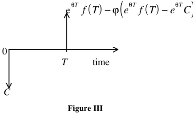
Therefore, if the nominal value of the pre tax net receipt h(T) is also indexed, i.e. h(T) = eθΤf(T), we have a situation that will be called of full indexation, and the cash flow associated with the investment, as expressed in current prices, is as depicted in Figure III
eθT
f T
( )
−
ϕ
(
e
θTf T
( )
−
e C
θT)
T time
Figure III
Cash-Flow in the Case of Full Indexation
9
Thus, as measured in constant prices, as referred to the date of the investment, the present value function to be maximized is:
F(T) = - C + e−RT
{
(
1
−
ϕ
) ( )
f T
+
ϕ
C
}
(17)It is then obvious that the optimal duration does not depend on the inflation rate θ.
c) partial indexation
Concluding the analysis, let us now consider the case where while the investment value is indexed for tax purposes, the nominal value of the pre tax net receipt h(T) is not. In this situation,
assuming that h(T) > CeθT, for T>0, it follows that the cash flow associated with the investment, as expressed in current prices, is as depicted in Figure IV.1
T time
C
Figure IV
Cash-Flow in the Case of Partial Indexation
In terms of constant prices, as expressed at the date of the investment, the correspondent present value is:
F(T) = - C + e− +(R θ)T
{
(
1
−
ϕ
)
h T
( )
+
ϕ
Ce
θT}
(18)
1
Note that, more generally, the value of the tax is given by max
{
0
;
ϕ
(h(T)
-
Ce
θT)
}
0
with
( ) ( ) ( ) ( ) ( )
{
(
)
}
( )dF T
dT
h T
R
h T
R Ce
e
T R T
=
−
′
−
+
−
− +1
ϕ
θ
ϕ
θ θ (19)Therefore, the optimal duration T* has to satisfy the following equation:
(
1−ϕ) ( ) (
(
h T′ − R+θ) ( )
h T)
−R Ceϕ θT =0 (20)On the other hand, as
( )
{
(
) ( ) (
(
) ( )
)
}
( )d F T
dT
Th T
R
h T
R Ce
e
T R T
2 2
1
=
−
′′
−
+
′
−
− + * * **
*
ϕ
θ
θ ϕ
θ θ(21)
T* will be indeed the optimal duration if
(
1−ϕ) ( ) (
(
h T′′ * − R+θ) ( )
h T′ *)
−θ ϕR CeθT* <0 (22)Also, differentiating (20), holding constant R and ϕ , we have that:
(
) ( )
(
) ( ) (
(
) ( )
)
dT
d
h T
T
R Ce
h T
R
h T
R Ce
T T
*
*
*
*
*
* *θ
ϕ
ϕ
ϕ
θ
θ ϕ
θ
θ
=
−
+
−
′′
−
+
′
−
1
1
(23)11
IV. Conclusion
References
Allen, R. G. D., 1938. Mathematical Analysis for Economists (St. Martin’s Press, New York).
Baumol, William J., 1972. Economic Theory and Operations Analysis, 3rd ed. (Prentice – Hall, Inc., Englewood Cliffs, N.J.).
Barbosa, Fernando de Holanda, 1993. La Indización de Los Activos Financieros: La Experiência Brasileña, in Luis Felipe Jiménez, Editor. Indización de Activos Financieros : Experiências Latinoamericanas - Argentina, Brasil, Colombia, Chile y Uruguay (Proyecto conjunto CEPAL/Gobierno de Holanda, SRV Impressos S.A., Santiago, Chile).
Bierman, Harold Jr. an Seymour Smidt, 1993. The Capital Budgeting Decision, 8th ed. (Macmillan Publishing Co., New York).
Brenner, Menachem and Itzak Venetia, 1983. The Effects of Inflation and Taxes on Growth Investments and Replacement Policies, Journal of Finance 38, 1519 - 1528.
de Faro, Clovis, 1996. The Effect of Taxes on Growth Investments: A Note, Revista de Análisis Económico 11, 139-142
Fishlow, Albert, 1974. Indexing Brazilian Style: Inflation Without Tears?, Brookings Papers on Economic Activity 1, 261-280.
Henderson, James M. and Richard E. Quandt, 1971. Microeconomic Theory: a Mathematical Approach, 2nd ed. (McGraw – Hill Book Co., New York).
Hirshleifer, J., 1970. Investment, Interest and Capital (Prentice-Hall, Inc., Englewood Cliffs, N.J.)
13
Simonsen, Mario Henrique, 1983. Indexation: Current Theory and the Brazilian Experience, in Rudiger Dornbusch and M. H. Simonsen, Editors. Inflation, Debt and Indexation (The MIT Press, Cambridge, Massachusetts).
Simonsen, Mario Henrique, 1995. 30 Anos de Indexação (Editora da Fundação Getulio Vargas, Rio de Janeiro, RJ.).
Varian, Hal R., 1990. Intermediate Microeconomics: a Modern Approach, 2nd ed. (W. W. Norton & Co., Inc., New York).