A model for simulating the timelines of field operations at a European scale for use in complex dynamic models

(1)

BGD

9, 10583–10614, 2012

A model for simulating the timelines of field

operations

N. J. Hutchings et al.

Title Page

Abstract Introduction

Conclusions References

Tables Figures

◭ ◮

Back Close

Full Screen / Esc

Printer-friendly Version Interactive Discussion

Discussion

P

a

per

|

Dis

cussion

P

a

per

|

Discussion

P

a

per

|

Discussio

n

P

a

per

|

Biogeosciences Discuss., 9, 10583–10614, 2012 www.biogeosciences-discuss.net/9/10583/2012/ doi:10.5194/bgd-9-10583-2012

Biogeosciences Discussions

This discussion paper is/has been under review for the journal Biogeosciences (BG). Please refer to the corresponding final paper in BG if available.

A model for simulating the timelines of

field operations at a European scale for

use in complex dynamic models

N. J. Hutchings1, G. J. Reinds2, A. Leip3, M. Wattenbach4,*, J. F. Bienkowski5, T. Dalgaard1, U. Dragosits6, J. L. Drouet7, P. Durand8, O. Maury7, and

W. de Vries9

1

Aarhus University, Department of Agroecology, Blichers All ´e 20, 8830 Tjele, Denmark

2

Alterra, Wageningen University and Research Centre, P.O. Box 47, 6700 AA Wageningen, The Netherlands

3

European Commission – DG Joint Research Centre, Institute for Environment and Sustainability, Via E. Fermi 2749, 21027 Ispra (VA), Italy

4

Institute of Biological and Environmental Sciences, School of Biological Sciences, University of Aberdeen, 23 St Machar Drive, Aberdeen, AB24 3UU, Scotland, UK

5

IAFE PAS, Poznan, Poland

6

CEH Edinburgh, Bush Estate, Penicuik, Midlothian EH26 0QB, Scotland, UK

7

INRA-AgroParisTech, UMR EGC, Thiverval-Grignon, France

8

INRA, UMR 1069 Soil AgroHydrosystems spatialisation, 35000 Rennes, France

9

(2)

BGD

9, 10583–10614, 2012

operations

Title Page

Tables Figures

◭ ◮

Back Close

Full Screen / Esc

Discussion

P

a

per

|

Dis

cussion

P

a

per

|

Discussion

P

a

per

|

Discussio

n

P

a

per

|

*

now at: Helmholtz Centre Potsdam, GFZ German Research Centre For Geosciences, Section 5.4 Hydrology, Telegrafenberg, 14473 Potsdam, Germany

Received: 29 June 2012 – Accepted: 3 July 2012 – Published: 9 August 2012

Correspondence to: N. J. Hutchings (nick.hutchings@agrsci.dk)

(3)

BGD

9, 10583–10614, 2012

operations

Title Page

Tables Figures

◭ ◮

Back Close

Full Screen / Esc

Discussion

P

a

per

|

Dis

cussion

P

a

per

|

Discussion

P

a

per

|

Discussio

n

P

a

per

|

Abstract

Complex dynamic models of carbon and nitrogen are often used to investigate the con-sequences of climate change on agricultural production and greenhouse gas emissions from agriculture. These models require high temporal resolution input data regarding the timing of field operations. This paper describes the Timelines model, which predicts 5

the timelines of key field operations across Europe. The evaluation of the model sug-gests that it is broadly capable of simulating the timing of field operations for a range of arable crops at different locations. Systematic variations in the date of harvesting and in the timing of the first application of N fertiliser to winter crops need to be corrected and the prediction of soil workability and trafficability might enable the prediction of 10

ploughing and applications of solid manure in preparation for spring crops. The data concerning the thermal time thresholds for sowing and harvesting underlying the model should be updated and extended to a wider range of crops.

1 Introduction

Complex dynamic models of carbon and nitrogen provide an insight into the interac-15

tions between agricultural management and the biotic/abiotic processes within agro-ecosystems. This is particularly true when investigating the possible consequences of climate change on greenhouse gas emissions from agriculture, since climate impacts occur at the process scale. However, obtaining appropriate values for parameters and driving variables presents investigators with a challenge; such models typically contain 20

a large number of parameters and operate with a temporal resolution of one day, so require input data with a high temporal resolution. Furthermore, it is relevant to con-ducting such investigations at a high spatial resolution because the predicted changes in response to climate change vary regionally as a function of land use and soil proper-ties (De Vries et al., 2012). Whilst it can be reasonably argued that some parameters 25

(4)

BGD

9, 10583–10614, 2012

operations

Title Page

Tables Figures

◭ ◮

Back Close

Full Screen / Esc

Discussion

P

a

per

|

Dis

cussion

P

a

per

|

Discussion

P

a

per

|

Discussio

n

P

a

per

|

this is not true for the driving variables. On a given field, meteorological variables (e.g. temperature, rainfall) and field operations (ploughing, sowing, fertilization, harvesting) are the main driving variables. There are good agronomic reasons why farmers take the weather into account when making decisions concerning field operations. For exam-ple, applying N fertiliser too much in advance of sowing could result in a low fertilisation 5

efficiency, if rainfall leads to the N being leached below the rooting zone or creates con-ditions that encourage denitrification. As a consequence, the timing is likely to vary in response to both year-to-year differences in weather and long-term changes in climate. The mechanisms driving both the direct emissions of greenhouse gases (GHG), such as N₂O and their indirect emissions (e.g. by NH₃emission and deposition and by 10

NO₃ leaching) are sensitive to short-term weather conditions (van Groeningen et al., 2005). Complex agroecosystem models attempt to describe these mechanisms, so researchers wishing to use them at the European scale must estimate agricultural management in the past and future. There has been significant progress regarding the collation of high-spatial resolution meteorological data for the past and the pre-15

diction of future climate (New et al., 2002; Klok and Klein Tank, 2009). In contrast, there has been less progress towards obtaining realistic field operation data at the Eu-ropean scale. Since such data cannot be obtained using automated techniques (e.g. from remote sensing), this requires the use of expensive standardised survey methods. Consequently, these data are often not available for the past or present in Europe, so 20

a purely statistical modelling approach to predicting the timing of past and future field operations is not possible.

The need for location-specific driving variables has been recognized for many years. The Crop Growth Modelling System (CGMS; http://www.marsop.info/marsopdoc/ cgms92/) of the EU Joint Research Centre was begun in the early 1990s (see van 25

(5)

BGD

9, 10583–10614, 2012

operations

Title Page

Tables Figures

◭ ◮

Back Close

Full Screen / Esc

Discussion

P

a

per

|

Dis

cussion

P

a

per

|

Discussion

P

a

per

|

Discussio

n

P

a

per

|

were generated by relating these events to thermal time and an interpolation proce-dure. Additional conditions, related to the likely soil moisture content, were also im-posed.

Part of the NitroEurope EU integrated research project (www.nitroeurope.eu) fo-cussed on the simulation of N₂O emissions and carbon sequestration from European 5

agriculture, for the period 1971–2030. This included the use of complex dynamic C and N crop and soil models at a high spatial resolution across Europe; nearly 42 000 rela-tively homogenous spatial units called NCUs (NitroEurope Calculation Units) based on an overlay of administrative units at NUTS2 (Statistical Office of the European Com-munities, 2003), soil mapping units according to the classes within the Soil Geographic 10

Database of the European Commission (http://eusoils.jrc.ec.europa.eu/esdb archive/ ESDBv2/fr intro.htm), and slope classes (i.e. 0–2 %, 2–8 %, 8–15 %, 15–25 %,>_{25 %),}

calculated on the basis of the Catchment Characterisation and Modelling Digital Ele-vation Model, (CCM 250 DEM). In addition a criterion on altitude was imposed limiting the difference in the average altitude of polygons in each NCU to 200 m. The models 15

used were DNDC-EUROPE (Leip et al., 2008), Mobile DNDC (De Bruijn et al., 2009) and DailyDayCent (Del Grosso et al., 2006). Given that over this 60 yr period there have been marked changes in climate already and further changes are predicted, the use of time-averaged field operation data was not considered appropriate for model input. While these models have the ability to predict the timing of one or more field 20

operations, one of the objectives of the exercise undertaken in the NitroEurope project was to compare the results of the different complex dynamic models. To avoid biasing the results towards a particular model, the driving variables needed to be generated independently.

Three models were used in the preparation of input data to these dynamic models 25

(6)

BGD

9, 10583–10614, 2012

operations

Title Page

Tables Figures

◭ ◮

Back Close

Full Screen / Esc

Discussion

P

a

per

|

Dis

cussion

P

a

per

|

Discussion

P

a

per

|

Discussio

n

P

a

per

|

manures applied to each crop and the annual deposition of N from the atmosphere, for each location in each year (De Vries et al., 2011). The third model simulated the timing (timelines) of field operations on each crop at each location in each year, and the use of field-scale measures to mitigate greenhouse gas emissions.

In this paper, we describe this latter model and compare the results with data that 5

was collected as part of the same project.

2 Methods

The methodology for the Timelines model was developed by a process of trial and error. In addition to a description of the final methodology, we include in this section a description of developments that proved not to be suitable for the operational model. 10

This is not only to provide an explanation of the methodology finally adopted, but also to alert anyone contemplating modifications or improvements to the methodology of the pitfalls that might lie in their way.

2.1 Specifications of the timelines model

The data to be generated were the timing of tillage, sowing, fertilisation with mineral 15

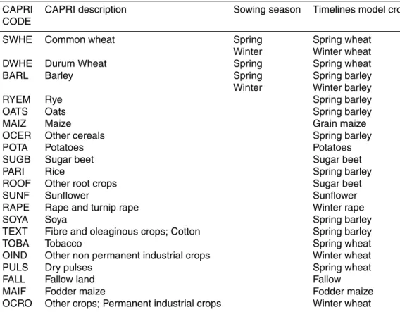
fertiliser and manure and harvesting. Timelines of field operations needed to be gen-erated for all crops and all NCUs to be simulated. The former was defined here to be all arable crops included in the CAPRI model (Britz and Witzke, 2008; see Table 1 below). Furthermore, although CAPRI does not distinguish between spring and winter cropping, the crop generator adds this information. The model requires data at an ad-20

equate spatial resolution at the European scale, for timelines to be generated at the daily scale, and to be consistent for multiple years. This latter constraint was imposed to support initialisation of the organic matter pools of the soil modules in the ecosystem models (“spinning up”) and simulation runs of su_fficient duration such that changes in soil C sequestration could be modelled.

(7)

BGD

9, 10583–10614, 2012

operations

Title Page

Tables Figures

◭ ◮

Back Close

Full Screen / Esc

Discussion

P

a

per

|

Dis

cussion

P

a

per

|

Discussion

P

a

per

|

Discussio

n

P

a

per

|

The major assumption behind the Timelines model is that the sowing and harvesting dates of crops can be related to accumulated air temperature, and that these two events can be used to frame all other field operations. It is also assumed that agronomic logic can be used to place the timing of ploughing, N fertilisation and manuring operations relative to these dates. More specifically, this logic assumes that farmers time fertilisa-5

tion and manuring operations to maximise nitrogen use efficiency for crop production. In both cases, it was accepted beforehand that these were gross simplifications. How-ever, they permitted the generation of timelines with the minimum of empirical input data, namely air temperature.

2.2 Sowing and harvesting

10

Although data concerning the timing of field operations are collected to varying extents in countries across Europe, to our knowledge, the data used in the CGMS represents the only Europe-wide harmonised dataset available. This dataset was constructed us-ing observations of the sowus-ing, ripenus-ing and harvestus-ing dates made in the early 1990s for a range of crops at locations across Europe. The values were subsequently interpo-15

lated onto the 50×50 km MARS meteorological grid to give complete coverage of the areas where these crops were grown. However, the CGMS uses a single dataset for all years, an approach that we considered inadequate for use in our study, since there have been important trends in the climate over the period we wished to consider. Fur-thermore, the range of crops considered was more limited than the range we wished 20

to include in our modelling.

To make the sowing and harvesting dates responsive to differences in the seasonal climate between years, we used a thermal time approach. The thermal time is the sum of the product of the time in days and the difference between the air temperature and a base temperature, below which temperature is ignored i.e. ifτ_t _{is the thermal time}

25

(8)

BGD

9, 10583–10614, 2012

operations

Title Page

Tables Figures

◭ ◮

Back Close

Full Screen / Esc

Discussion

P

a

per

|

Dis

cussion

P

a

per

|

Discussion

P

a

per

|

Discussio

n

P

a

per

|

τ_t₌ t

X

k₌t₀

max ((θ_k₋θ_b_{) , 0)}

Whereθ_k _{is the air temperature (Celsius) on day}k_{. For simplicity, a value of zero was}

used for the base temperature throughout this work.

We first back-calculated the reference thermal time for the data in the CGMS dataset, 5

using the average air temperature data for the years 1985 to 1995. The mean daily air temperature was estimated by averaging the minimum and maximum daily air tem-peratures in the MARS dataset. This reference thermal time data was then used to calculate sowing and harvesting data across Europe for the historical climate record for 1971 to 2000 and to the predicted climate for the period 2000 to 2030 (using the A1 10

climate scenario) to generate the predicted crop-specific dates of sowing and harvest-ing across Europe. The meteorological data for the period 1970–2000 was obtained by combining the MARS grid weather (Orlandi and Van der Goot, 2003) with interpolated monthly climate data at 10′

×10′spatial resolution (Mitchell et al., 2004). For the period 2001–2030, recent simulations from the REMO model (Jacob, 2001) were provided 15

by the Max-Planck-Institute for Meteorology, Germany. Meteorological data were pro-cessed as described in Cameron et al. (2012) and de Vries et al. (2012). The CGMS dataset includes the following crops: winter wheat, winter barley, winter rape, spring barley, spring rape, spring wheat, sugar beet, potatoes, sunflower, grain maize and fodder maize. To enable the crops not included in the CGMS dataset to be modelled, 20

replacement crops were identified (Table 1).

Initial simulations with the model as described above identified a number of issues. The first was that in a small number of instances, either the sowing or the harvesting dates were not available for a crop in the MARS grid where the crop generator pre-dicted that the crop would be cultivated. In this situation, the search was progressively 25

(9)

BGD

9, 10583–10614, 2012

operations

Title Page

Tables Figures

◭ ◮

Back Close

Full Screen / Esc

Discussion

P

a

per

|

Dis

cussion

P

a

per

|

Discussion

P

a

per

|

Discussio

n

P

a

per

|

A second problem was that on some occasions when the crop generator predicted the planting of a winter crop, the sowing date for these crops was before the harvesting date for the preceding crop. This was probably due to a combination of the relatively short period between harvesting and sowing, and uncertainty introduced into the deter-mination of the dates by the original CGMS interpolation procedure and the further data 5

processing described above. However, for forage maize, which is commonly harvested later than other arable crops and is rarely followed by winter cereals, this appeared to be due to a failure to constrain the crop generator accordingly. The solution adopted in the problematic instances was to advance the crop harvesting to a date five days prior to the sowing date of the winter crop. This was to allow the winter crop sufficient time 10

to become established and thereby avoid unrealistically low crop coverage during the winter period.

A third problem encountered was that with climate warming, the sowing dates of win-ter cereals advanced towards mid-summer. This resulted in the autumn-sown cereals being predicted to enter the winter at an unrealistically advanced development stage. 15

The solution adopted here was to abandon the use of the thermal time concept to determine the sowing date of winter cereals and to rely on the original, static dataset.

2.3 Other field operations

In general, the timing of other field operations is assumed to be closely related to the sowing date. However, for applications of mineral fertiliser and animal slurry to winter 20

cereals, the timing is related to the start of the growing season.

Ploughing in preparation for all crops was assumed to occur three days prior to the sowing date.

The timing of manure applications was assumed to vary according to the manure type. The N in solid manure is mainly in the organic form, so must be mineralised 25

(10)

BGD

9, 10583–10614, 2012

operations

Title Page

Tables Figures

◭ ◮

Back Close

Full Screen / Esc

Discussion

P

a

per

|

Dis

cussion

P

a

per

|

Discussion

P

a

per

|

Discussio

n

P

a

per

|

and winter crops were there for placed five days prior to the sowing date (i.e. two days before ploughing).

For spring crops, applications of animal slurry coincided with the application of solid manure, whereas for winter crops the applications were timed to coincide with the start of the growing season. The start of the growing season for the winter crops at a given 5

location was equated to the sowing date for spring barley at the same location.

The timing offertiliser applicationswas assumed to be designed to promote efficient use of the fertiliser N, so the annual amount is applied in two applications. The first application was assumed to consist of 20 % of the annual amount and to be made 5 days prior to sowing (spring crops) or at the start of the growing season (winter crops). 10

The second application, of the remaining 80 %, was assumed to be made after 20 % of the growing season has elapsed. This distribution was intended to match the supply of N to the absorption potential of the crop, bearing in mind that manure N will often be supplied prior to sowing.

This timing was subsequently modified to ensure that the second fertiliser application 15

did not take place within 21 days of harvesting.

2.4 Atmospheric N deposition

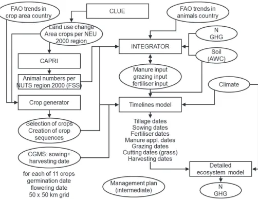
The annual atmospheric N deposition is calculated on the basis of NH₃and NO_x emis-sions from agro-ecosystems calculated by the INTEGRATOR model (De Vries et al., 2011, 2012), combined with historic EMEP data on NOx emissions and an

emission-20

deposition matrix for NH₃ and NO_x, derived from the EMEP model (Simpson et al., 2003; EMEP, 2009). This INTEGRATOR input was output from the Timelines model as a single operation, timed on 1 January each year. The ecosystem models then distributed this N equally on a daily basis. For 2020 the non-agricultural N emission scenarios was used that reflects current legislation, that was developed for the The-25

(11)

BGD

9, 10583–10614, 2012

operations

Title Page

Tables Figures

◭ ◮

Back Close

Full Screen / Esc

Discussion

P

a

per

|

Dis

cussion

P

a

per

|

Discussion

P

a

per

|

Discussio

n

P

a

per

|

2.5 Implementation

The model was implemented in the C++ programming language, using the Eclipse development environment and the GNU C++compiler. The software is freely available at http://afoludata.jrc.ec.europa.eu/, together with instructions for use and details of the input and output file formats. The input from the crop generator and INTEGRATOR 5

models consisted of separate, annual data concerning:

– The crop grown.

– The application of N as ammonium and nitrate.

– The amounts of N and C applied in solid manure and slurry originating from cattle, pigs, sheep/goats and poultry (solid manure only).

10

– The N deposited from the atmosphere.

The data concerning a particular field operation consisted of the date when the opera-tion was initiated, together with a variable number of operaopera-tion-specific supplementary data. For example, the supplementary data associated with a manure application were the amount and type of animal manure applied, while for harvesting, the supplementary 15

data included the method used to harvest a crop. Estimated crop yield was required by a number of the ecosystem models; this was provided by the fertilisation/manure model and the information was attached to the harvesting operations. Full technical details can be found at http://afoludata.jrc.ec.europa.eu/index.php/dataset/detail/219.

3 Evaluation

20

3.1 Data source

(12)

BGD

9, 10583–10614, 2012

operations

Title Page

Tables Figures

◭ ◮

Back Close

Full Screen / Esc

Discussion

P

a

per

|

Dis

cussion

P

a

per

|

Discussion

P

a

per

|

Discussio

n

P

a

per

|

established in a number of European countries. Of these, the timings of field opera-tions from three landscape areas were extracted for evaluating the Timelines model. The landscapes were in Bjerringbro, Denmark (56.3◦_{N, 9.7}◦_{E), Turew, Naizin, France}

(48.0◦_{N, 2.8}◦_{W) and Poland (52.0}◦_{N, 16.8}◦_{E) (Fig. 2).}

The data collected by survey from these study areas included dates of field opera-5

tions for a single crop year (2007–2008), which can be compared with the simulated results by the Timelines model. The survey results were stored in a Microsoft Access database for each landscape. All field operation data for each case study area were exported from the Access database in XML format, with individual operations subse-quently extracted. Finally, since the data did not appear to be normally distributed, 10

median dates for the operations were calculated. For fertilisation events, which are as-sumed to occur twice per growing season in the Timelines model, the partitioning of fertilisation events between the first and second application periods was made visually from plotted data. In some instances, it was clear that there was only one application period, in which case the second application date was not calculated.

15

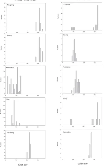
Two example datasets, one for a winter crop (winter wheat in France) and one for a spring crop (potatoes in Poland) are shown in Fig. 3.

3.2 Comparison of recorded and predicted field operations

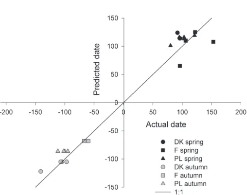
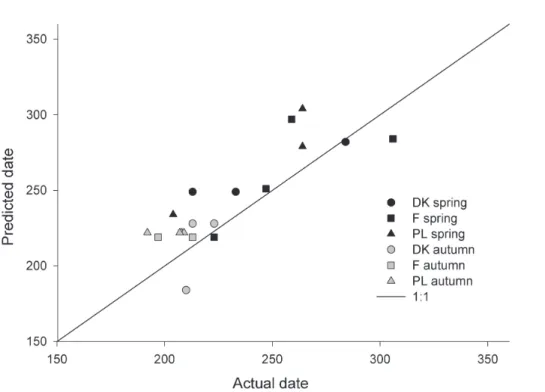
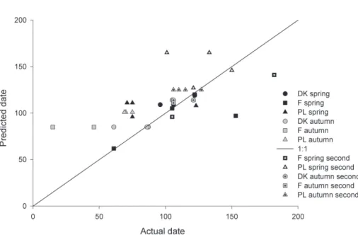
The actual and predicted data from the NitroEurope landscape study areas concerning sowing, harvesting, ploughing, fertilisation, application of slurry and application of solid 20

manure are shown in the Figs. 4–8 and in more detail in the Tables S1 to S6, respec-tively (see Supplement). The number of field operations recorded varied considerably between areas and crops; crops for which there were five or fewer records were omit-ted. Two spring crops (spring barley and maize) and two winter crops (winter barley and winter wheat) were adequately represented in all three landscapes. For these crops, 25

(13)

BGD

9, 10583–10614, 2012

operations

Title Page

Tables Figures

◭ ◮

Back Close

Full Screen / Esc

Discussion

P

a

per

|

Dis

cussion

P

a

per

|

Discussion

P

a

per

|

Discussio

n

P

a

per

|

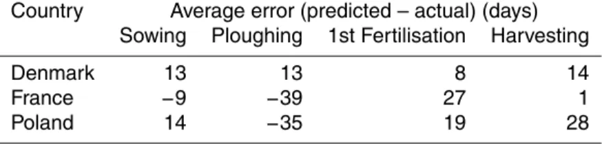
For sowing, there is some evidence to suggest that the absolute magnitude of the di_fference between the predicted and median dates decreased with the number of records, reflecting the effect of the large range of dates recorded in each landscape (Table 1). There were major differences between the landscapes regarding the perfor-mance of the model. In Denmark, the model predicted a sowing date consistently later 5

than recorded. This trend was visible for most winter crops, across all landscapes. For the crops that can be compared between locations (Table 2), there is a consistent ten-dency for the predicted date to be later than the recorded date. For harvesting, there are large errors for both sugar and fodder beet and possibly also for maize. For the crops that can be compared (Table 2), the predicted harvesting dates for both spring 10

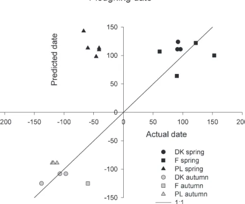
and winter barley are later than those recorded. For ploughing in preparation for the sowing of spring crops, the model assumes that the ploughing also occurs the spring. However, for some crops (in Poland, for most crops), the ploughing occurred predom-inantly in the autumn. This can be seen in Table 3, where data for the field operations for the selected crops are averaged by landscape. For the application of mineral N fer-15

tiliser, there are errors in the prediction for maize. The predicted application dates for winter crops are consistently too late in the season (Table 2). For a number of crops, the distribution of dates was clearly monotonic and no second application period could be calculated. There were fewer data for the date of slurry and solid manure applica-tions, so these operations are not included in Tables 2 and 3. The notable features are 20

instances of slurry application in the autumn and of solid manure applications in the spring in Denmark, in association with winter crops.

4 Discussion

4.1 Performance of the model

There was a clearer relationship between the predicted and measured sowing dates for 25

(14)

BGD

9, 10583–10614, 2012

operations

Title Page

Tables Figures

◭ ◮

Back Close

Full Screen / Esc

Discussion

P

a

per

|

Dis

cussion

P

a

per

|

Discussion

P

a

per

|

Discussio

n

P

a

per

|

the date of sowing will be similar for all spring crops, so it is likely that other factors play an important role in determining the date of sowing e.g. soil moisture constraints on trafficability and workability or competition for labour and machinery. The only excep-tion is maize, which as a C4 plant is more temperature sensitive than the remaining, predominantly C3 crops. A later sowing date later than for other crops would therefore 5

be expected and this was the case in France and Poland (but not Denmark). In contrast to the spring, the timing of the sowing of winter crops is less likely to be constrained by soil conditions, since the soil is likely to be drier at this time. The autumn sowing period is mainly constrained on one side by the harvesting date of the previous crop and on the other, by the wish to avoid the crop developing so extensively before enter-10

ing the winter that there is an increased risk of damage by frost, snow or disease. The predicted dates for harvesting were about 10–20 days later than recorded in practice (Fig. 5). This is the reverse of the expected situation; the CGMS data are based on the dates for ripening rather than harvesting, so the need on occasions for other conditions to be satisfied (e.g. to allow cereal crops to dry sufficiently for storage) would be ex-15

pected to delay harvesting past the time of ripening. This could be due to changes in the crop varieties grown since the 1990s or to interpolation errors in the thermal time in the CGMS or in the meteorological data.

The observations indicate that ploughing in preparation for the sowing of spring crops can occur both in the spring and autumn (Fig. 6). Anecdotal evidence from Poland and 20

France suggests that ploughing in the autumn is common on soils that are likely to be too wet to ploughing the spring (either due to a high clay content or high water table); the chances that the soils are more workable in the autumn may be higher. The model might therefore be improved by taking into account the effect of soil moisture conditions on workability and trafficability. However, this would require the addition of a soil water 25

(15)

BGD

9, 10583–10614, 2012

operations

Title Page

Tables Figures

◭ ◮

Back Close

Full Screen / Esc

Discussion

P

a

per

|

Dis

cussion

P

a

per

|

Discussion

P

a

per

|

Discussio

n

P

a

per

|

The assumption that the first application of mineral fertiliser to winter crops in the spring coincides with the start of plant growth (equated in the model to the sowing date of spring barley) appears to be incorrect; according to the landscape surveys, the fer-tiliser applications are made somewhat earlier than that date (Fig. 7). For those winter crops that can be compared across landscapes, the actual date of first application ap-5

pears to be about one month before that predicted by the model. The assumption in the model that the annual fertiliser inputs are split between two application dates is some-times incorrect. For maize, this may be a systematic e_ffect; the growth of maize occurs over a shorter and later period than for the C3 crops, so farmers may consider that the risk of losing fertiliser N by leaching or denitrification is sufficiently low that a single 10

application date is adequate. The current model does not take into account any interac-tion between the mineral fertiliser and organic manure applicainterac-tions; a farmer wishing to manage nutrients efficiently would manage both sources simultaneously. For example, if applying a substantial quantity of organic manure in the spring, the farmer may omit the first spring application of fertiliser N. An additional source of error in the present 15

study is that visually estimating the boundaries of the periods for the first and second applications of fertiliser was sometimes difficult; a more objective, statistical approach would be preferable.

The solid manure applications associated with spring cropping that are sometimes observed to be made in the previous autumn (Fig. 8) can probably be explained by 20

the desire to incorporate these manures and hence link the date of application to the timing of ploughing (see above). There is also some evidence that solid manure may be applied in the spring to winter crops.

4.2 Scope for improvement

The current assessment of the Timelines model suggests that it broadly fulfils the func-25

(16)

BGD

9, 10583–10614, 2012

operations

Title Page

Tables Figures

◭ ◮

Back Close

Full Screen / Esc

Discussion

P

a

per

|

Dis

cussion

P

a

per

|

Discussion

P

a

per

|

Discussio

n

P

a

per

|

effect of the trafficability and workability of clay-rich or poorly-drained soils. The in-troduction of a soil moisture model would allow such conditions to be predicted. The timing of the first application of N fertiliser to winter crops needs to be brought forward by about one month.

Predicting the timing of applications of manure is particularly di_fficult. Unless obliged 5

or persuaded to value the nutrients contained in manures, farmers are likely to choose to apply them when labour and machinery are least busy and when soil conditions permit tra_fficking with application equipment i.e. on frozen soil during the winter, with-out regard to nutrient recovery. This leads to an extended manure application period. However, the progressive enforcement of the EU Nitrates Directive has led to the intro-10

duction of obligatory balanced fertilisation and restrictions on autumn and winter appli-cations of organic manures over an increasingly large area of the EU (CEC, 2002), both of which will tend to concentrate manure applications into the spring period. Since the Timelines model assumes good nutrient management, continued enforcement of the Nitrates Directive, implementation of the EU Water Framework Directive and the effect 15

of increasing energy prices on the cost of mineral fertiliser N, is likely that the pre-dictions regarding manure applications will improve with time. However, further work is necessary if the Timelines model is to be used in connection with the modelling of historical production or nutrient flows.

The model is currently not able to accommodate double cropping. This makes the 20

model less applicable to Southern European countries. Furthermore, since climate change may lead to a northward migration of the geographic boundary of the area where double cropping is feasible, this constraint is likely to grow with time.

4.3 Future

The advisability of using the Timelines model when using complex ecosystem mod-25

(17)

BGD

9, 10583–10614, 2012

operations

Title Page

Tables Figures

◭ ◮

Back Close

Full Screen / Esc

Discussion

P

a

per

|

Dis

cussion

P

a

per

|

Discussion

P

a

per

|

Discussio

n

P

a

per

|

operations, the model may be useful. However, it will often be preferable for weather-dependent timing of field operations to be introduced into the ecosystem models them-selves. This removes the risk of internal inconsistencies in the modelling system e.g. when the Timelines model predicts that a crop should be harvested while the ecosys-tem model predicts that it is not yet ripe. The chances of such inconsistencies arising 5

would increase if a soil moisture model were included in the Timelines model.

The evaluation undertaken here was limited by the resources available within the NitroEurope project and there is scope for a more thorough analysis of the data from the NitroEurope landscapes, e.g. concerning the relationships between different field operations. Similar data also exist from other EU or national research projects; given 10

the scarcity of such data, there is a need to locate and collate these datasets, and undertake a more detailed analysis than was possible here. This might in particular allow the evaluation to be extended into Southern Europe.

The current model is heavily reliant on the empirical data on sowing and harvesting dates currently used within CGMS. The range of crops included is limited and the data 15

are now quite old, so do not reflect modern crop varieties. In addition, the data do not reflect the effect of climate change and crop breeding on the movement of the northern boundary for the cultivation of certain crops, such as maize. As ecosystem models become more complex and are increasingly used to inform policymaking, it is important for the quality of the predictions from those models that the quality of the 20

driving variables keeps pace. This argues for further work on predicting the timing of field operations but not least, for improved empirical data.

5 Conclusions

The evaluation of the Timelines model suggests that it is broadly capable of simulating the timing of field operations for a range of arable crops at different locations across 25

(18)

BGD

9, 10583–10614, 2012

operations

Title Page

Tables Figures

◭ ◮

Back Close

Full Screen / Esc

Discussion

P

a

per

|

Dis

cussion

P

a

per

|

Discussion

P

a

per

|

Discussio

n

P

a

per

|

addition of a soil moisture module, capable of simulating workability and trafficability, might enable the Timelines model to predict occasions when ploughing and applica-tions of solid manure in preparation for spring crops are made in the previous autumn. Finally, the data concerning the thermal time thresholds for sowing and harvesting that underlie the model are old and consider too few crops; the use of complex ecosystem 5

models would benefit if these data could be updated and expanded.

Supplementary material related to this article is available online at: http://www.biogeosciences-discuss.net/9/10583/2012/

bgd-9-10583-2012-supplement.pdf.

Acknowledgements. The authors would like to thank The European Commission and Aarhus 10

University for financially supporting the NitroEurope research project (www.NitroEurope.eu), within which the presented research was undertaken.

References

Amann, M., Asman, W., Bertok, I., Cofala, J., Heyes, C., Klimont, Z., Sch ¨opp, W., and Wag-ner, F.: Cost-effective emission reductions to meet the environmental targets of the Thematic 15

Strategy on Air Pollution under different greenhouse gas constraints, NEC Scenario Analysis Report Nr. 5, IIASA, Laxenburg, Austria, 2007.

Britz, W. and Witzke H.-P.: CAPRI model documentation 2008: Version 2, available at: http: //www.capri-model.org, last access: 29 June 2012.

CCM 250 DEM: EuroLandscape/Agri-Environment Catchment Characterisation and Modelling 20

Activity, Land Management Unit, Institute for Environment and Sustainability, EC-Joint Re-search Centre, 250 Meter DEM, compiled on the basis of data acquired from data providers and national mapping agencies over Europe, 2004.

Commission of the European Communities: Implementation of Council Directive 91/676/EEC concerning the protection of waters against pollution caused by nitrates from agricultural 25

(19)

BGD

9, 10583–10614, 2012

operations

Title Page

Tables Figures

◭ ◮

Back Close

Full Screen / Esc

Discussion

P

a

per

|

Dis

cussion

P

a

per

|

Discussion

P

a

per

|

Discussio

n

P

a

per

|

LexUriServ/LexUriServ.do?uri=COM:2002:0407:FIN:EN:PDF (last access: 29 June 2012),

2002.

Cameron, D. R., van Oijen, M., Butterbach-Bahl, K., Haas, E., Heuvelink, G., Grote, R., Kiese, R., Kuhnert, M., Kros, J., Reinds, G. J., Reuter, H. I., Schelhaas, M. J., de Vries, W., Werner, C., and Yeluripati, J. B.: Environmental change impacts on the C- and N-cycle of 5

European forests: a model comparison study, Biogeosciences, submitted, 2012.

de Bruijn, A. M. G., Butterbach-Bahl, K., Blagodatsky, S., and Grote, R.: Model evaluation of different mechanisms driving freeze-thaw N₂O emissions, Agr. Ecosyst. Environ., 133, 196– 207, 2009.

Del Grosso, S. J. , Parton, W. J., Mosier, A. R., Walsh, M. K., Ojima, D. S., and Thornton, P. E.: 10

DAYCENT national-scale simulations of nitrous oxide emissions from cropped soils in the United States, J. Environ. Qual., 35, 1451–1460, 2006.

De Vries, W., Leip, A., Reinds, G. J., Kros, J., Lesschen, J. P., and Bouwman, A. F.: Comparison of land nitrogen budgets for European agriculture by various modeling approaches, Environ. Pollut., 159, 3253–3267, 2011.

15

De Vries, W., Kros, J., Reinds, G. J., Wieggers, H. J. J., Velthof, G. L., Oudendag, D. A., Less-chen, J. P., Schelhaas, M. J., Perez Soba, M., Rienks, W., de Winter, W. P., Uijterwijk, M., van den Akker, J., Leip, A., Bakker, M. M., Verburg, P. H., Neumann, K., Liski, J., Eickhout B., and Bouwman, A. F.: Assessment of nitrogen and greenhouse gas fluxes at the European scale in response to land cover, livestock and land management change, Agr. Ecosyst. Environ., 20

in preparation, 2012.

European Commission: European Soil Database (version V2.0), CD-ROM EUR 19945 EN, March 2004, European Commission, Directorate General Joint Research Centre, Institute for Environment and Sustainability, Ispra, Italy, 2004.

Jacob, D.: A note to the simulation of the annual and interannual variability of the water budget 25

over the Baltic Sea drainage basin, Meteorol. Atmos. Phys., 77, 61–74, 2001.

Klok, E. J. and Klein Tank, A. M. G.: Updated and extended European dataset of daily climate observations, Int. J. Climatol., 29, 1182, doi:10.1002/joc.1779, 2009.

Leip, A., Marchi, G., Koeble, R., Kempen, M., Britz, W., and Li, C.: Linking an economic model for European agriculture with a mechanistic model to estimate nitrogen and carbon losses 30

from arable soils in Europe, Biogeosciences, 5, 73–94, doi:10.5194/bg-5-73-2008, 2008. Mitchell, T. D., Carter, T. R., Jones, P. D., Hulme, M., and New, M. A.: Comprehensive Set of

(20)

BGD

9, 10583–10614, 2012

operations

Title Page

Tables Figures

◭ ◮

Back Close

Full Screen / Esc

Discussion

P

a

per

|

Dis

cussion

P

a

per

|

Discussion

P

a

per

|

Discussio

n

P

a

per

|

(1901–2000) and 16 Scenarios (2001–2100), Tyndall Centre for Climate Change Research, University of East Anglia, Norwich, UK, 2004.

New, M., Lister, D., Hulme, M., and Makin, I.: A high-resolution data set of surface climate over global land areas, Clim. Res., 21, 1–25, 2002.

Orlandi, S. and Van der Goot, E.: Technical description of

in-5

terpolation and processing of meteorological data in CGMS,

available at: http://mars.jrc.ec.europa.eu/mars/Bulletins-Publications/

Technical-description-of-interpolation-and-processing-of-meteorological-data-in-CGMS, European Commission, DG JRC, Agrifish Unit (last access: 6 August 2012), 2003.

Simpson, D., Fagerli, H., Jonson, J. E., Tsyro, S., Wind, P., and Tuovinen, J.-P.: Transbound-10

ary Acidification, Eutrophication and Ground Level Ozone in Europe PART I. Unified EMEP Model Description, Norwegian Meteorological Institute, EMEP Status Report, 2003.

Statistical O_ffice of the European Communities (EUROSTAT): The Geographic Information Sys-tem of the European Commission (GISCO) reference database: Version: 07/2003, Brussels, 2003.

15

Sutton, M. A., Nemitz, E., Erisman, J. W., Beier, C., Butterbach Bahl, K., Cellier, P. de Vries, W., Cotrufo, F., Skiba, U., Di Marco, C. Jones, S., Laville, P., Soussana, J. F., Loubet, B., Twigg, M., Famulari, D., Whitehead, J., Gallagher, M. W., Neftel, A., Flechard, C. R., Herr-mann, B., Calanca, P. L., Schjoerring, J. K., Daemmgen, U., Horvath, L., Tang, Y. S., Em-mett, B. A., Tietema, A., Pe ˜nuelas, J., Kesik, M., Brueggemann, N., Pilegaard, K., Vesala, T., 20

Campbell, C. L., Olesen, J. E., Dragosits, U., Theobald, M. R., Levy, P., Mobbs, D. C., Milne, R., Viovy, N., Vuichard, N., Smith, J. U., Smith, P., Bergamaschi, P., Fowler, D., and Reis, S.: Challenges in quantifying biosphere-atmosphere exchange of nitrogen species, En-viron. Pollut., 150, 125–139, 2007.

van Diepen, K. and Boogaard, H.: History of CGMS in the MARS project, Agro Informatica, 22, 25

11–14, 2009.

van Groenigen, J. W., Velthof, G. L., van der Bolt, F. J. E., Vos, A., and Kuikman, P. J.: Seasonal variation in N₂O emissions from urine patches: e_ffects of urine concentration, soil compaction and dung, Plant Soil, 273, 15–27, 2005.

Willekens, A., Van Orshoven, J., and Feyen, J.: Estimation of the phenological calendar, Kc-30

(21)

BGD

9, 10583–10614, 2012

operations

Title Page

Tables Figures

◭ ◮

Back Close

Full Screen / Esc

Discussion

P

a

per

|

Dis

cussion

P

a

per

|

Discussion

P

a

per

|

Discussio

n

P

a

per

|

the European Communities, Space Applications Institute, MARS-project, Ispra, Italy, 31 pp., 1998.

Wattenbach, M., Hillier, J., Schartner, T., Hattermann, F., Wechsung, F., van Oijen, M., de Vries, W., Reinds, G. J., Kros, J., Yeluripati, J., Kuhnert, M., Hutchings, N. J., Kiese, R., Werner, C., Butterbach Bahl, K., Leip, A., and Smith, P.: A generic probability-based algo-5

(22)

BGD

9, 10583–10614, 2012

operations

Title Page

Tables Figures

◭ ◮

Back Close

Full Screen / Esc

Discussion

P

a

per

|

Dis

cussion

P

a

per

|

Discussion

P

a

per

|

Discussio

n

P

a

per

|

Table 1.CAPRI crops and their Timelines equivalents.

CAPRI CAPRI description Sowing season Timelines model crop

CODE

SWHE Common wheat Spring Spring wheat

Winter Winter wheat

DWHE Durum Wheat Spring Spring wheat

BARL Barley Spring Spring barley

Winter Winter barley

RYEM Rye Spring barley

OATS Oats Spring barley

MAIZ Maize Grain maize

OCER Other cereals Spring barley

POTA Potatoes Potatoes

SUGB Sugar beet Sugar beet

PARI Rice Spring barley

ROOF Other root crops Sugar beet

SUNF Sunflower Sunflower

RAPE Rape and turnip rape Winter rape

SOYA Soya Spring barley

TEXT Fibre and oleaginous crops; Cotton Spring barley

TOBA Tobacco Spring wheat

OIND Other non permanent industrial crops Winter wheat

PULS Dry pulses Spring wheat

FALL Fallow land Fallow

MAIF Fodder maize Fodder maize

(23)

BGD

9, 10583–10614, 2012

operations

Title Page

Tables Figures

◭ ◮

Back Close

Full Screen / Esc

Discussion

P

a

per

|

Dis

cussion

P

a

per

|

Discussion

P

a

per

|

Discussio

n

P

a

per

|

Table 2.Average error in predicted date of field operations for selected crops.

Crop Average error (predicted – actual) (days)

Sowing Ploughing 1st Fertilisation Harvesting

Spring barley 3 −76 12 21

Maize 11 20 −4 5

Winter barley 8 −12 42 22

(24)

BGD

9, 10583–10614, 2012

operations

Title Page

Tables Figures

◭ ◮

Back Close

Full Screen / Esc

Discussion

P

a

per

|

Dis

cussion

P

a

per

|

Discussion

P

a

per

|

Discussio

n

P

a

per

|

Table 3.Average error in predicted date of field operations for the selected crops, by landscape.

Country Average error (predicted – actual) (days)

Sowing Ploughing 1st Fertilisation Harvesting

Denmark 13 13 8 14

France −9 −39 27 1

(25)

BGD

9, 10583–10614, 2012

operations

Title Page

Tables Figures

◭ ◮

Back Close

Full Screen / Esc

Discussion

P

a

per

|

Dis

cussion

P

a

per

|

Discussion

P

a

per

|

Discussio

n

P

a

per

|

(26)

BGD

9, 10583–10614, 2012

operations

Title Page

Tables Figures

◭ ◮

Back Close

Full Screen / Esc

Discussion

P

a

per

|

Dis

cussion

P

a

per

|

Discussion

P

a

per

|

Discussio

n

P

a

per

|

(27)

BGD

9, 10583–10614, 2012

operations

Title Page

Tables Figures

◭ ◮

Back Close

Full Screen / Esc

Discussion

P

a

per

|

Dis

cussion

P

a

per

|

Discussion

P

a

per

|

Discussio

n

P

a

per

|

(28)

BGD

9, 10583–10614, 2012

operations

Title Page

Tables Figures

◭ ◮

Back Close

Full Screen / Esc

Discussion

P

a

per

|

Dis

cussion

P

a

per

|

Discussion

P

a

per

|

Discussio

n

P

a

per

|

(29)

BGD

9, 10583–10614, 2012

operations

Title Page

Tables Figures

◭ ◮

Back Close

Full Screen / Esc

Discussion

P

a

per

|

Dis

cussion

P

a

per

|

Discussion

P

a

per

|

Discussio

n

P

a

per

|

(30)

BGD

9, 10583–10614, 2012

operations

Title Page

Tables Figures

◭ ◮

Back Close

Full Screen / Esc

Discussion

P

a

per

|

Dis

cussion

P

a

per

|

Discussion

P

a

per

|

Discussio

n

P

a

per

|

(31)

BGD

9, 10583–10614, 2012

operations

Title Page

Tables Figures

◭ ◮

Back Close

Full Screen / Esc

Discussion

P

a

per

|

Dis

cussion

P

a

per

|

Discussion

P

a

per

|

Discussio

n

P

a

per

|

(32)

BGD

9, 10583–10614, 2012

operations

Title Page

Tables Figures

◭ ◮

Back Close

Full Screen / Esc

Discussion

P

a

per

|

Dis

cussion

P

a

per

|

Discussion

P

a

per

|

Discussio

n

P

a

per

|