Investigation of effects of varying model inputs on mercury deposition estimates in the Southwest US

(1)

ACPD

12, 10273–10304, 2012

E_ffects of varying model inputs on mercury deposition

estimates

T. Myers et al.

Title Page

Abstract Introduction

Conclusions References

Tables Figures

◭ ◮

Back Close

Full Screen / Esc

Printer-friendly Version

Interactive Discussion

Discussion

P

a

per

|

Dis

cussion

P

a

per

|

Discussion

P

a

per

|

Discussio

n

P

a

per

|

Atmos. Chem. Phys. Discuss., 12, 10273–10304, 2012 www.atmos-chem-phys-discuss.net/12/10273/2012/ doi:10.5194/acpd-12-10273-2012

Atmospheric Chemistry and Physics Discussions

This discussion paper is/has been under review for the journal Atmospheric Chemistry and Physics (ACP). Please refer to the corresponding final paper in ACP if available.

Investigation of e

_ff

ects of varying model

inputs on mercury deposition estimates

in the Southwest US

T. Myers1, R. D. Atkinson2, O. R. Bullock Jr.3, and J. O. Bash3

1

ICF International, 101 Lucas Valley Rd., San Rafael, CA 94903, USA 2

Office of Water, US Environmental Protection Agency, Washington, DC, USA

3

National Exposure Research Laboratory, US Environmental Protection Agency, Research Triangle Park, NC, USA

Received: 6 March 2012 – Accepted: 3 April 2012 – Published: 20 April 2012

Correspondence to: T. Myers (tmyers@icfi.com)

(2)

ACPD

12, 10273–10304, 2012

estimates

T. Myers et al.

Title Page

Tables Figures

◭ ◮

Back Close

Full Screen / Esc

Discussion

P

a

per

|

Dis

cussion

P

a

per

|

Discussion

P

a

per

|

Discussio

n

P

a

per

|

Abstract

The Community Multiscale Air Quality (CMAQ) model version 4.7.1 was used to sim-ulate mercury wet and dry deposition for a domain covering the contiguous United States (US). The simulations used MM5-derived meteorological input fields and the US Environmental Protection Agency (EPA) Clear Air Mercury Rule (CAMR)

emis-5

sions inventory. Using sensitivity simulations with different boundary conditions and tracer simulations, this investigation focuses on the contributions of boundary concen-trations to deposited mercury in the Southwest (SW) US. Concenconcen-trations of oxidized mercury species along the boundaries of the domain, in particular the upper layers of the domain, can make significant contributions to the simulated wet and dry deposition

10

of mercury in the SW US. In order to better understand the contributions of boundary conditions to deposition, inert tracer simulations were conducted to quantify the relative amount of an atmospheric constituent transported across the boundaries of the domain at various altitudes and to quantify the amount that reaches and potentially deposits to the land surface in the SW US. Simulations using alternate sets of boundary

concen-15

trations, including estimates from global models (Goddard Earth Observing System-Chem (GEOS-System-Chem) and the Global/Regional Atmospheric Heavy Metals (GRAHM) model), and alternate meteorological input fields (for different years) are analyzed in this paper. CMAQ dry deposition in the SW US is sensitive to differences in the atmo-spheric dynamics and atmoatmo-spheric mercury chemistry parameterizations between the

20

global models used for boundary conditions.

1 Introduction

Regional scale simulations of mercury deposition must rely on boundary concentra-tions to account for fluxes of species, in particular the various mercury species, into the modeling domain from the remainder of the globe. In the North American Mercury

25

(3)

ACPD

12, 10273–10304, 2012

estimates

T. Myers et al.

Title Page

Tables Figures

◭ ◮

Back Close

Full Screen / Esc

Discussion

P

a

per

|

Dis

cussion

P

a

per

|

Discussion

P

a

per

|

Discussio

n

P

a

per

|

deposition simulated by regional scale models depends strongly on the initial and boundary concentrations of mercury compounds used for the regional scale simula-tions. Pongprueska et al. (2008) found that the influence of the initial conditions was much weaker than the influence of boundary concentrations. Therefore, in order to in-terpret the results from regional scale simulations of mercury deposition, it is important

5

to understand the influence that the boundary concentrations have on the simulated mercury deposition.

In this study, the results obtained in the NAMMIS study are expanded by considering, in addition to the effect of using alternate boundary concentrations, the effect of sev-eral other factors on simulated mercury deposition. Specifically, use of meteorological

10

inputs for a different year; use of an alternative global model as a source of boundary concentrations for the regional scale simulations; changes in the high altitude bound-ary concentrations; and increased vertical resolution in the regional scale modeling domain are examined. In addition, tracer simulations are used to clarify how the simu-lated mercury species are transported from the boundary to areas in the domain that

15

are impacted by the boundary concentrations.

We use a 36 km resolution regional scale grid covering most of North America, but some of the analyses are focused on locations in the Southwest (SW) US where CMAQ model simulations showed high levels of total Hg dry deposition compared to other models considered in the NAMMIS (Bullock et al., 2008).

20

2 Background on simulations

The Community Multiscale Air Quality (CMAQ) model version 4.7.1 (Foley et al., 2011) was used to simulate mercury wet and dry deposition for a domain covering the con-tiguous US and parts of Mexico and Canada. Simulations were made with CMAQ 4.7.1 without the elemental Hg-NO3 reaction. Sommar et al. (1997) reported an oxidation

25

(4)

ACPD

12, 10273–10304, 2012

estimates

T. Myers et al.

Title Page

Tables Figures

◭ ◮

Back Close

Full Screen / Esc

Discussion

P

a

per

|

Dis

cussion

P

a

per

|

Discussion

P

a

per

|

Discussio

n

P

a

per

|

However, the rate constent reported by Sommar et al. (1997) was not statistically dif-ferent from 0 and the assumed products are thermodynamically unfavorable (Hynes et al., 2009). The inclusion of this reaction mechanism in CMAQ 4.7 was found to over-estimate the modeled wet deposition when compared to MDN observations (116 % normalized mean bias in January and February 2002 simulations and 11 % normalized

5

mean bias (NMB) in July and August 2002 simulations) and found to result in ambient low, sub 1 ng m−3_{GEM concentrations, in hemispheric CMAQ simulations. The removal}

of GEM oxidation by the NO3radical reduced the January and February wet deposition

bias (31 % NMB) and introduced a negative bias in the July and August 2002 simula-tions (−23 % NMB but decreased the normalized mean error by from 44 % to 39 %).

10

CMAQ 4.7.1 with this change to the chemical mechanism was found to simulate wet deposition well when compared to MDN observations and CAMx simulations (Baker and Bash, 2012). This GEM oxidation pathway was removed in CMAQ 5.0. Total dry deposition of mercury presented here includes only deposition of divalent gas mercury and particulate mercury. The deposition of elemental mercury simulated by CMAQ is

15

not included in the analyses. The bidirectional deposition algorithm for elemental mer-cury in CMAQ was not used in this study, and it is therefore assumed that deposition of elemental mercury would be roughly offset by subsequent evasion of elemental mer-cury. This study therefore focusses on the deposition of divalent forms of mercury which would contribute to a net increase in the mercury loadings of the a_ffected land areas.

20

All simulations reported here used meteorological input files derived from the Fifth Generation Mesoscale Model (MM5; Grell et al., 1994) simulations. The 2001 simula-tions used meteorological files and emissions files from the NAMMIS. The emissions files were developed from the US EPA Clean Air Mercury Rule (CAMR) emissions inventory (EPA, 2005), and these emissions files were also used for the 2005

simula-25

(5)

ACPD

12, 10273–10304, 2012

estimates

T. Myers et al.

Title Page

Tables Figures

◭ ◮

Back Close

Full Screen / Esc

Discussion

P

a

per

|

Dis

cussion

P

a

per

|

Discussion

P

a

per

|

Discussio

n

P

a

per

|

reported in Sect. 7. CMAQ ready meteorological files for 2005 with 14 vertical layers were also derived from MM5 outputs. These 2005 files were acquired from EPA and had been used in past EPA studies (EPA, 2009).

The 14-layer vertical grid configuration used for the CMAQ simulations reported here is the same as was used for the CMAQ simulations reported in NAMMIS: a

sigma-5

pressure based vertical coordinate system with model top at 10 kPa. The 34-layer grid configuration used in simulations in Sect. 7 used the same model top with additional sigma layers. The correspondence of layers for the 14 and 34 layer grid systems is shown in Table 1.

The 2002 CMAQ simulation used 14-layer meteorological files derived from MM5

10

simulations and emissions from the 2002 National Emissions Inventory (http://www. epa.gov/ttn/chief/net/critsummary.html).

Boundary and initial conditions for mercury species derived from GEOS-Chem (Bey et al., 2001) and the Global/Regional Atmospheric Heavy Metals (GRAHM) (Dastoor and Larocque, 2004; Ariya et al., 2004) are those developed by participants in

NAM-15

MIS: GEOS-Chem by the Massachusetts Institute of Technology and Harvard Uni-versity (Selin et al., 2007), and GRAHM by Environment Canada. Initial and bound-ary concentrations of all species other than mercury were derived from the NAMMIS GEOS-Chem simulation and were the same for all simulations reported here.

Concentrations of oxidized mercury species along the boundaries of the domain,

20

in particular the upper layers of the domain, can make significant contributions to the simulated wet and dry deposition of mercury in the SW US. In order to better under-stand the contributions of boundary conditions to deposition, inert tracer simulations were conducted to quantify the relative amount of atmospheric constituents transported across the boundaries of the domain at various altitudes and to quantify the amount

25

(6)

ACPD

12, 10273–10304, 2012

estimates

T. Myers et al.

Title Page

Tables Figures

◭ ◮

Back Close

Full Screen / Esc

Discussion

P

a

per

|

Dis

cussion

P

a

per

|

Discussion

P

a

per

|

Discussio

n

P

a

per

|

Simulations were initiated on 21 June and were run through 31 July 2001 and 2005. Deposition totals are for 1 July through 31 July. Additional simulations were run for February and July 2002 that used boundary concentrations based on a CMAQ northern-hemispheric simulation.

In the sections below, simulation results for the following cases will be discussed:

5

use of alternative sets of boundary concentrations for mercury species; effect of alter-ing boundary concentrations of mercury at high altitudes; tracers showalter-ing the contribu-tion of boundary regions to surface concentracontribu-tions; effect of alternate meteorology on estimated deposition (using 2001 vs. 2005 meteorological data); and effect of higher vertical resolution on tracer results.

10

3 Alternate sets of boundary concentrations

3.1 GEOS-Chem vs. GRAHM boundary conditions

The effect of global transport of mercury is embodied in the boundary concentrations used for a regional simulation. The choice of these boundary concentrations can have a significant effect of the simulated estimates of deposition of atmospheric pollutants

15

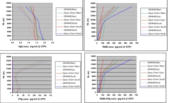
(Schere et al., 2012). This comparison examines simulated total dry deposition and simulated mercury total wet deposition using two different sets of boundary concen-trations for mercury derived from the global models GEOS-Chem and GRAHM. These CMAQ simulations were run with 14 vertical layers. The vertical variation in the bound-ary concentrations is shown in Fig. 1.

20

Although the elemental mercury (Hg0) concentrations derived from the Chem results and from the GRAHM results are similar near the surface, the GEOS-Chem boundary conditions are more than double the GRAHM boundary conditions at altitudes above 12 000 m. At lower altitudes, the reactive gaseous mercury (RGM) boundary conditions derived from GEOS-Chem, at around 80 pg m−3_{, are higher}

25

than the boundary conditions derived from GRAHM (about 30 pg m−3

(7)

ACPD

12, 10273–10304, 2012

estimates

T. Myers et al.

Title Page

Tables Figures

◭ ◮

Back Close

Full Screen / Esc

Discussion

P

a

per

|

Dis

cussion

P

a

per

|

Discussion

P

a

per

|

Discussio

n

P

a

per

|

above 10 000 m, the GEOS-Chem boundary conditions on the north boundary range from 200–600 pg m−3

while the GRAHM boundary conditions range from about 100– 350 pg m−3

. On the south boundary, however, the GEOS-Chem boundary conditions reach a maximum of only roughly 100 pg m−3 _{at the top of the domain, while the}

GRAHM boundary conditions reach 400 pg m−3

at the top of the domain. The GRAHM

5

and GEOS-Chem boundary conditions for RGM are for the most part within about 50 % of each other at higher altitudes on the west and east boundaries, covering a range of concentrations from about 50 pg m−3

at 10 000 m to roughly 300 pg m−3

at the top of the domain. Particle bound mercury (PHg) is only about 1 pg m−3

in the GEOS-Chem derived boundary conditions compared to the GRAHM derived boundary conditions

10

which have concentrations of about 25 pg m−3 _{up to 10 000 m and 125 pg m}−3 _{at the}

top of the domain. The final panel of Fig. 1 shows the sum of RGM and PHg in order to compare the total divalent mercury present on the boundaries. In general, the total di-valent mercury boundary conditions derived from the two global models are closer than the separate components. GEOS-Chem derived boundary conditions remain higher at

15

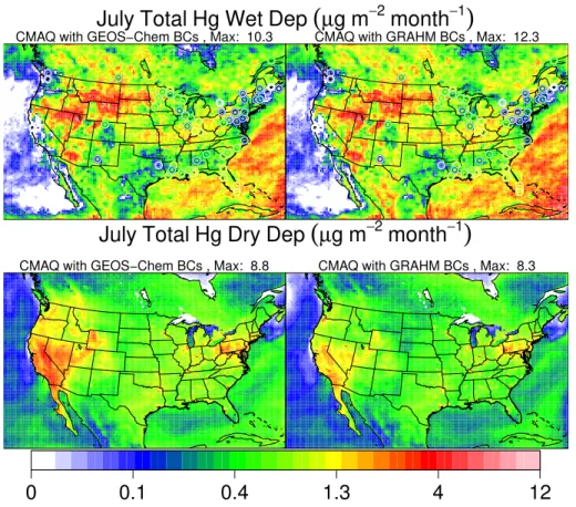
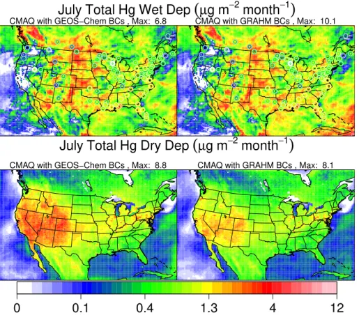
low altitudes on the west boundary and lower at high altitudes on the south boundary. Figure 2 demonstrates the substantially di_fferent estimates of mercury deposition that can result from the different boundary conditions. In particular, dry deposition in some parts of California and Nevada drops from 4 µg m−2_month−1 _{using the}

GEOS-Chem boundary conditions to about 1.5 µg m−2_month−1 _{using the GRAHM}

bound-20

ary conditions. Simulated wet deposition of mercury in some areas of Arizona is about 1.3 µg m−2_month−1 _{using the GEOS-Chem boundary conditions but increases}

to 1.5 µg m−2_month−1_{using the GRAHM boundary conditions.}

3.2 Adjusted GEOS-Chem boundary conditions

In this section, wet and dry mercury deposition simulated by CMAQ for February 2002

25

(8)

ACPD

12, 10273–10304, 2012

estimates

T. Myers et al.

Title Page

Tables Figures

◭ ◮

Back Close

Full Screen / Esc

Discussion

P

a

per

|

Dis

cussion

P

a

per

|

Discussion

P

a

per

|

Discussio

n

P

a

per

|

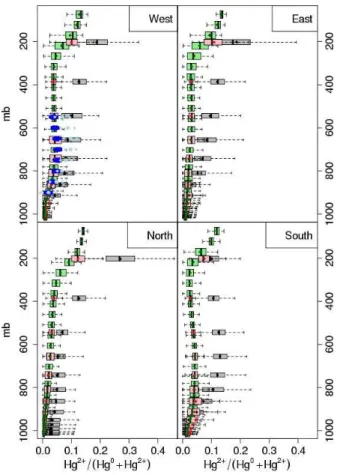
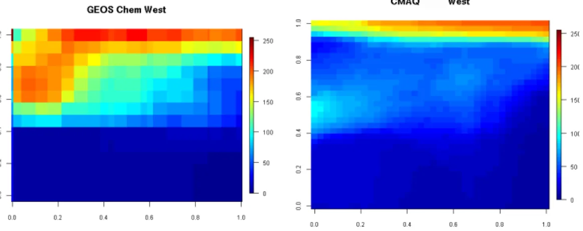
non-mercury species constant in the boundary conditions between the simulations. The fraction of divalent oxidized mercury, Hg(II), to total mercury, THg, was compared be-tween the April monthly mean 2005 CMAQ hemispheric run, the GEOS-Chem bound-ary conditions, and measurements taken aloft from Schwarzendruber et al. (2009). GEOS-Chem boundary conditions were several factors larger than CMAQ boundary

5

conditions above the 800 mb level, Figs. 3 and 4. To develop new boundary concentra-tions, the CMAQ hemispheric layer structure was processed to 14 layers and the me-dian CMAQ hemispheric oxidized fraction of the gas phase Hg, RGM/(GEM+RGM), was used to adjust GEOS-Chem GEM and Hg concentrations to match the fraction in the oxidized phase while preserving the total gas phase Hg for the 14 vertical pressure

10

levels. This adjustment was assumed to be constant in time and was applied to bound-ary concentrations derived from a 2002 GEOS-Chem model simulation for the Janubound-ary through February and July through August 2002 simulations. The total gaseous mer-cury at each pressure level in the GEOS-Chem boundary conditions was preserved, e.g. if CMAQ hemispheric runs estimated lower RGM concentrations the reduction in

15

RGM in the Chem boundary conditions was allocated to GEM. The GEOS-Chem PHg was not adjusted in these boundary conditions. These new boundary con-ditions agree better with the profiles measured by Schwarzendruber et al. (2009) below the 800 mb pressure level and are lower than the observations above that, Fig. 3.

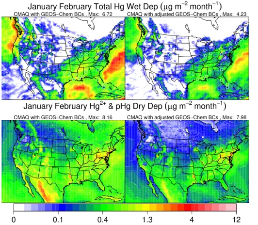
The changes in boundary concentrations are illustrated in Fig. 4. CMAQ simulations

20

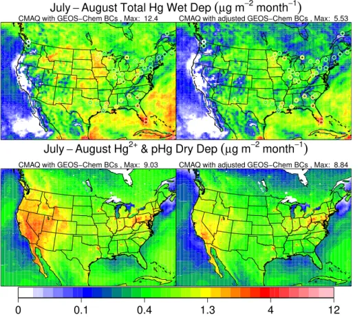
for January, February, July and August 2002 were made. The CMAQ simulations were run at 36 km horizontal grid resolution on a contiguous US domain. The simulated dry and wet deposition results for February 2002 are presented in Fig. 5. The sensitivity of wet deposition and dry deposition is nearly proportional to the reduction of Hg(II) in the boundary conditions at the 800 to 500 mb pressure levels (−48 % and −40 % in

25

January and February and−38 % and−29 % in July and August respectively).

(9)

ACPD

12, 10273–10304, 2012

estimates

T. Myers et al.

Title Page

Tables Figures

◭ ◮

Back Close

Full Screen / Esc

Discussion

P

a

per

|

Dis

cussion

P

a

per

|

Discussion

P

a

per

|

Discussio

n

P

a

per

|

domain, particularly in the SW US and northern portion of the domain where reductions in dry deposition are greater than 50 %. Simulated wet deposition is also lower using the adjusted boundary conditions. The relative reduction in wet deposition is largest (∼50 %) in the SW US, but the absolute change is small (∼0.5 µg m−2month−1) due to lower precipitation rates. The comparisons in Fig. 5 show the strong influence of

5

boundary concentrations on the mercury deposition simulated by CMAQ.

4 Alternate meteorology

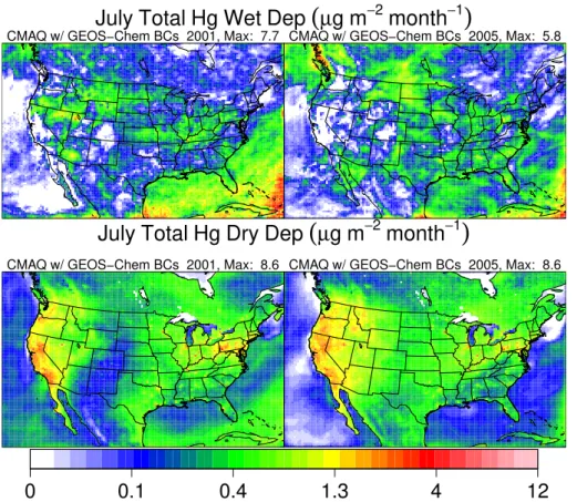
In this section, comparisons are made between the July 2001 and July 2005 simula-tions. Using an alternate set of meteorological inputs while maintaining other inputs constant shows that the response of the CMAQ simulation to changes in the boundary

10

concentrations is also considerable using inputs other than the 2001 meteorology. The CMAQ simulations for July 2005 were made with meteorological input files also derived from MM5 outputs. Boundary conditions and emissions were the same as those in the 2001 simulations. As with the 2001 CMAQ simulations, two sets of simulations were made, one with boundary conditions based on the GEOS-Chem global model and the

15

other with boundary conditions based on the GRAHM global model.

The wet and dry deposition of divalent mercury simulated by CMAQ for the July 2005 time period using the GEOS-Chem and GRAHM derived boundary conditions are shown in Fig. 6. The simulated dry deposition of mercury using the July 2005 meteorological files was 50 to 100 % higher in the SW US than the simulated dry

de-20

position of mercury using the July 2001 meteorological files, with a greater difference when the GEOS-Chem boundary conditions were used (compare to Fig. 2). Simulated wet deposition of mercury shows large spatial variations between the two simulations using different meteorological inputs since wet deposition is driven by the presence of rainfall. The response of the model to the use of different boundary concentrations is

25

(10)

ACPD

12, 10273–10304, 2012

estimates

T. Myers et al.

Title Page

Tables Figures

◭ ◮

Back Close

Full Screen / Esc

Discussion

P

a

per

|

Dis

cussion

P

a

per

|

Discussion

P

a

per

|

Discussio

n

P

a

per

|

conditions regardless of whether 2001 or 2005 meteorology was used. The response in simulated dry deposition of mercury is more pronounced using the 2005 meteorology than the 2001 meteorology. Although peak simulated wet deposition of mercury may be higher or lower using either sets of boundary conditions, in general the wet deposition of mercury is lower over the contiguous US using the GRAHM boundary conditions

5

compared to GEOS-Chem boundary conditions. This is most noticeable in the South-east (SE) US where simulated wet deposition is lower by about 50 % using the GRAHM boundary conditions compared to using the GEOS-Chem boundary conditions, while in the SW US the difference is consistently less than 50 %.

5 Effect of high altitude mercury boundary concentrations

10

In order to assess the e_ffects of the high altitude boundary concentrations on mercury deposition, boundary concentrations of all mercury species were zeroed out in the top two layers (i.e. layers 13 and 14) which corresponds to a height of approximately 5400 m and above. These simulations were made with the GEOS-Chem boundary conditions using both the 2001 and 2005 meteorology.

15

The simulated deposition in Fig. 7 can be compared directly to Figs. 2 and 6. Note that both wet deposition and dry deposition are reduced in both meteorological years. In the SW US, the model estimates substantially lower deposition of mercury when the upper layers of the boundary concentrations are set to zero for all mercury species. To see the influence of the upper layer mercury on deposition more clearly, the

dif-20

ferences between the simulations with and without the upper layer mercury boundary conditions were calculated and expressed as a percent contribution from the upper layer boundary conditions to deposition (Fig. 8).The strong influence of the higher alti-tude mercury boundary concentrations on the simulated deposition of mercury is clear from this figure. From 20 to 80 % of the simulated dry deposition of mercury in the

25

(11)

ACPD

12, 10273–10304, 2012

estimates

T. Myers et al.

Title Page

Tables Figures

◭ ◮

Back Close

Full Screen / Esc

Discussion

P

a

per

|

Dis

cussion

P

a

per

|

Discussion

P

a

per

|

Discussio

n

P

a

per

|

greater than for dry deposition. Over most of the SW US, more than 80 % of the sim-ulated wet deposition of mercury originates from the upper layer boundary conditions. Unlike other species that typically have low concentrations at higher altitude, relatively high concentrations of mercury at higher altitudes must be considered when setting boundary concentrations for model simulations.

5

6 Tracers showing upper tropospheric impact on surface concentrations

In order to assess whether the contributions of high altitude boundary concentrations to mercury deposition are primarily due to high mercury levels in the upper atmosphere or transport from the upper layers to lower layers, simulations were conducted with unit concentration tracers along each of the domain boundaries, broken down by model

10

layer. These simulations were conducted for the month of July using both 2001 and 2005 meteorology.

Preparation of the tracer simulations involved a minor modification to the CMAQ 4.7.1 code and preparation of initial and boundary concentration files that included tracer concentrations. The CMAQ “trac0” header files, such as “TR SPC.EXT”, are supplied

15

in the release version of the model with zero tracers. These files were modified to in-clude 26 tracers with names such as “TRAC1”, “TRAC2”, and so forth. These tracers were assigned to boundaries, initial concentrations and layers as shown in Table 2. For example, therefore, “TRAC12” was assigned unit concentration in layers 3 through 6 on the north boundary, and zero concentration elsewhere, including in the initial

con-20

centration file.

The spatial pattern of the contributions of the upper layers to surface layer is simi-lar for both sets of meteorological inputs (see Fig. 9), although the peak contribution from the upper layers is higher using the 2005 meteorology. The greater simulated dry deposition of mercury using the 2005 meteorology appears to be at least in part a

re-25

(12)

ACPD

12, 10273–10304, 2012

estimates

T. Myers et al.

Title Page

Tables Figures

◭ ◮

Back Close

Full Screen / Esc

Discussion

P

a

per

|

Dis

cussion

P

a

per

|

Discussion

P

a

per

|

Discussio

n

P

a

per

|

concentrations, that the largest contribution to the lower layers from the upper layers occurs over the Rocky Mountains, which then spreads out to influence other parts of the domain.

At two locations in the domain, one in Arizona (grid cell (44, 45)) and one in California (grid cell (24, 51)), the influence of the upper layer boundaries was examined in more

5

detail. The green symbols in Fig. 10 show the locations subject to this more detailed examination. A breakdown of contributors to surface tracer concentrations is shown in Fig. 11. The influence of the upper boundaries on the surface is almost 50 % at the Arizona location, but is only about 30 % at the California location. The influence of the upper layers comes not only from the western boundary, but also from other boundaries

10

as well. In particular, a further breakdown shows that there is a strong influence from the south boundary. Conversely, the 2001 meteorological case shows a relatively small influence of the lower part of the western boundary at the Arizona location, although the upper part of the western boundary has a fairly large influence. These results could be due to different flow fields from the meteorology in these model simulations.

15

7 Tracers with increased vertical resolution impact on surface concentrations

The 14-layer simulations presented thus far include relatively limited vertical resolution in the upper layers. It is therefore of interest to determine if the influences of the upper layers may be exaggerated in the simulations due to this low resolution. An additional simulation was therefore conducted using meteorological files based on the same MM5

20

model runs for 2001 used for the tracer simulation in the previous section. The MM5 model runs used 34-layers. For the prior runs, the CMAQ ready meteorological files were processed to 14 layers, requiring degradation in vertical resolution, although the vertical extent of the MM5 domain was maintained. In this simulation, the CMAQ ready meteorological files retained all 34 layers of the MM5 output so the resolution was not

25

(13)

ACPD

12, 10273–10304, 2012

estimates

T. Myers et al.

Title Page

Tables Figures

◭ ◮

Back Close

Full Screen / Esc

Discussion

P

a

per

|

Dis

cussion

P

a

per

|

Discussion

P

a

per

|

Discussio

n

P

a

per

|

Tracers were defined in a manner similar to the methodology described for the 14-layer tracer simulation in Sect. 6. In this case, 52 tracers were used and covered the 34 layers included in this domain.

Using higher resolution meteorological files does not change the basic conclusions about the strong influence of upper layer boundaries on simulated surface layer

mer-5

cury concentrations. The area of the domain affected by upper layers is similar using either 14 or 34 layers (see Figs. 9a and 12). The peak influence of the upper layer boundaries is somewhat higher for the tracer concentration using the 34 layer mete-orological files. The breakdown of the influence of the boundaries at the locations in Arizona and California (Fig. 11) shows similar influence from the upper boundaries

10

overall to what is shown for 2001. The relative influence of west vs. other boundaries differs, however, depending on whether the 14 or 34 layer files are used.

8 Conclusions

CMAQ dry deposition in the SW US is sensitive to di_fferences in the atmospheric dy-namics and atmospheric mercury chemistry parameterizations of the global models

15

used for boundary conditions. Changes in estimates of boundary concentrations affect conclusions about the total amount of mercury deposition. This implies a large uncer-tainty in what is referred to as background mercury. The contribution from upper layers to wet and dry deposition of Hg is large regardless of global model used for boundary conditions. The magnitude of the boundary concentrations throughout the depth of the

20

modeling domain must be carefully considered given these sensitivities, not just within the boundary layer or mixed layer. Although the details of simulated deposition change with di_fferent meteorological years, the strong influence of the boundaries is present in all cases investigated, and the response to changes in boundary concentrations is similar. Localized mixing brings upper-level material to the surface. The influence of

25

(14)

ACPD

12, 10273–10304, 2012

estimates

T. Myers et al.

Title Page

Tables Figures

◭ ◮

Back Close

Full Screen / Esc

Discussion

P

a

per

|

Dis

cussion

P

a

per

|

Discussion

P

a

per

|

Discussio

n

P

a

per

|

the upper-level air mass with the lower-level air mass. The influence of the upper layer boundary conditions is not restricted to the western boundary; boundary conditions from upper layers along other boundaries can also have a strong influence at locations in the SW US. Over 80 % of the simulated wet deposition in parts of the SW US orig-inated from the upper layers of the boundary conditions. The model indicates that the

5

area that experiences the greatest amount of upper tropospheric transport of mercury to the surface is in the Rocky Mountains and that this influences other parts of the domain. Elevated levels of Hg(II) have been observed at high altitude monitoring sites and attributed to deep tropospheric mixing (Fa¨In et al., 2009) in agreement with these modeled results. Increasing the vertical resolution of the input fields used for the CMAQ

10

modeling does not reduce the influence of the upper layer boundary concentrations on the surface air mass in the SW US, although the simulation of the tracers is altered somewhat by the use of higher vertical resolution. The influence of Hg concentrations on the dry deposition from the free troposphere in CMAQ is in agreement with the model and measurement comparisons of Amos et al. (2012). These results may

par-15

tially explain the recently documented discrepancies between modeled and observed speciated mercury concentrations (Baker and Bash, 2012).

Supplementary material related to this article is available online at: http://www.atmos-chem-phys-discuss.net/12/10273/2012/

acpd-12-10273-2012-supplement.zip.

20

Disclaimer._{Although this work was reviewed by EPA and approved for publication, it may not}

(15)

ACPD

12, 10273–10304, 2012

estimates

T. Myers et al.

Title Page

Tables Figures

◭ ◮

Back Close

Full Screen / Esc

Discussion

P

a

per

|

Dis

cussion

P

a

per

|

Discussion

P

a

per

|

Discussio

n

P

a

per

|

References

Amos, H. M., Jacob, D. J., Holmes, C. D., Fisher, J. A., Wang, Q., Yantosca, R. M., Corbitt, E. S., Galarneau, E., Rutter, A. P., Gustin, M. S., Steffen, A., Schauer, J. J., Graydon, J. A., Louis, V. L. St., Talbot, R. W., Edgerton, E. S., Zhang, Y., and Sunderland, E. M.: Gas-particle

partitioning of atmospheric Hg(II) and its effect on global mercury deposition, Atmos. Chem.

5

Phys., 12, 591–603, doi:10.5194/acp-12-591-2012, 2012.

Ariya, P., Dastoor, A., Amyot, M., Schroeder, W., Barrie, L., Anlauf, K., Raofie, F., Ryzhkov, A., Davignon, D., Lalonde, J., and Steffen, A.: Arctic: A sink for mercury, Tellus, 56B, 397–403, 2004.

Baker, K. and Bash, J.: Regional scale photochemical model evaluation of total mercury wet

10

deposition and speciated ambient mercury, Atmos. Environ., 49, 151–162, 2012.

Bash, J. O.: Description and initial simulation of a dynamic bidirectional air-surface exchange model for mercury in Community Multiscale Air Quality (CMAQ) model, J. Geophys. Res., 115, D06305, doi:10.1029/2009JD012834, 2010.

Bey, I., Jacob, D., Yantosca, R., Logan, J., Field, D., Fiore, A., Li, Q., Liu, H., Mickley, L., and

15

Schultz, M.: Global modeling of tropospheric chemistry with assimilated meteorology: Model description and evaluation, J. Geophys. Res., 106, 23073–23095, 2001.

Bullock Jr., O., Atkinson, D., Braverman, T., Civerolo, K., Dastoor, A., Davignon, D., Ku, J., Lohman, K., Myers, T., Park, R., Seigneur, C., Selin, N., Sistla, G., and Vija-yaraghavan, K.: The North American Mercury Model Intercomparison Study (NAMMIS):

20

Study description and model-to-model comparisons, J. Geophys. Res., 113, D17310, doi:10.1029/2008JD009803, 2008.

Dastoor, A. and Larocque, Y.: Global circulation of atmospheric mercury: A modeling study, Atmos. Environ., 38, 147–161, 2004.

EPA: Emissions Inventory and Emissions Processing for the Clean Air Mercury Rule (CAMR),

25

EPA OAQPS, http://www.epa.gov/ttn/atw/utility/emiss inv oar-2002-0056-6129.pdf, 2005. EPA: Meteorological Modeling Performance Evaluation for the Annual 2005 Continental US

36-km Domain Simulation, EPA Office of Air Quality Planning and Standards (OAQPS), 2009.

Fa¨ın, X., Obrist, D., Hallar, A. G., Mccubbin, I., and Rahn, T.: High levels of reactive gaseous mercury observed at a high elevation research laboratory in the Rocky Mountains, Atmos.

30

(16)

ACPD

12, 10273–10304, 2012

estimates

T. Myers et al.

Title Page

Tables Figures

◭ ◮

Back Close

Full Screen / Esc

Discussion

P

a

per

|

Dis

cussion

P

a

per

|

Discussion

P

a

per

|

Discussio

n

P

a

per

|

Foley, K. M., Roselle, S. J., Appel, K. W., Bhave, P. V., Pleim, J. E., Otte, T. L., Mathur, R., Sarwar, G., Young, J. O., Gilliam, R. C., Nolte, C. G., Kelly, J. T., Gilliland, A. B., and Bash, J. O.: Incremental testing of the Community Multiscale Air Quality (CMAQ) modeling system version 4.7, Geosci. Model Dev., 3, 205–226, doi:10.5194/gmd-3-205-2010, 2010.

Grell, G., Dudhia, A., and Stauffer, D.: A description of the Fifth-Generation PennState/NCAR

5

Mesoscale Model (MM5). NCAR Technical Note NCAR/TN-398+STR, available at: http://

www.mmm.ucar.edu/mm5/doc1.html, 1994.

Hall, B.: The gas-phase oxidation of elemental mercury by ozone, Water Air Soil Pollut., 80, 301–315, 1995.

Hynes, A. J., Donohoue, D. L., Goodsite, M. E., and Hedgecock, I. M.: Our current

understand-10

ing of major chemical and physical processes affectinf mercury dynamics in the atmosphere

and at the air-water/terrestrial interfaces, in: Mercury Fate and Transport in the Global Atmo-sphere, edited by: Pirrone, N. and Mason, R., Springer, New York, 427–457, 2009.

Otte, T., Pouliot, G., Pleim, J., Young, J., Schere, K., Wong, D., Lee, P., Tsidulko, M., McQueen, J., Davidson, P., Mathur, R., Chuang, H., DiMego, G., and Seaman, N.: Linking the Eta model

15

with the Community Multiscale Air Quality (CMAQ) modeling system to build a national air quality forecasting system, Weather Forecast., 20, 367–384, 2005.

Pal, B. and Ariya, P.; Studies of ozone initiated reactions of gaseous mercury: kinetics, product studies and atmospheric implications, Environ. Sci. Technol., 38, 5555–5566, 2004.

Pongprueksa, P., Lin, C. J., Lindberg, S. E., Jang, C., Braverman, T., Bullock, O. R., Ho, T. C.,

20

and Chu, H. W.: Scientific uncertainties in atmospheric mercury models III: Boundary and initial conditions, model grid resolution, and Hg(II) reduction mechanism, Atmos. Environ., 42, 1828–1845, 2008.

Schere, K., Flemming, J., Vautard, R., Chemel, C., Colette, A., Hogrefe, C., Bessagnet, B., Meleux, F., Mathur, R., Roselle, S., Hu, R., Sokhi, R., Rao, S., and Galmarini, S.: Trace

25

gas/aerosol boundary concentrations and their impacts on continental-scale AQMEII model-ing domains, Atmos. Environ., in press, 2012.

Selin, N., Jacob, D., Park, R., Yantosca, R., Strode, S., Jaegle, L., and Ja_ffe, D.: Chemical cy-cling and deposition of atmospheric mercury: Global constraints from observations, J. Geo-phys. Res., 112, D02308, doi:10.1029/2006JD007450, 2007.

30

(17)

ACPD

12, 10273–10304, 2012

estimates

T. Myers et al.

Title Page

Tables Figures

◭ ◮

Back Close

Full Screen / Esc

Discussion

P

a

per

|

Dis

cussion

P

a

per

|

Discussion

P

a

per

|

Discussio

n

P

a

per

|

Subir, M., Ariya, P. A., and Dastoor, A. P.: A review of uncertainties in atmospheric modeling of mercury chemistry I. Uncertainties in existing kinetic parameters – Fundamental limitations and the importance of heterogeneous chemistry, Atmos. Environ., 45, 5664–5676, 2011. Swartzendruber, P., Jaffe, D., and Finley, B.: Development and first results of an aircraft-based,

high time resolution technique for gaseous elemental and reactive (oxidized) gaseous

mer-5

(18)

ACPD

12, 10273–10304, 2012

estimates

T. Myers et al.

Title Page

Tables Figures

◭ ◮

Back Close

Full Screen / Esc

Discussion

P

a

per

|

Dis

cussion

P

a

per

|

Discussion

P

a

per

|

Discussio

n

P

a

per

|

Table 1.Sigma-p layer definitions for 14-layer and 34-layer CMAQ simulations.

Layer No. in 14-layer grid Layer No. in 34-layer grid Sigma-p at layer top

1 1 0.995

2 2 0.99

3 0.985

3 4 0.98

5 0.97

4 6 0.96

7 0.95

5 8 0.94

9 0.93

10 0.92

6 11 0.91

12 0.9

13 0.88

7 14 0.86

15 0.84

16 0.82

8 17 0.8

18 0.77

9 19 0.74

20 0.7

10 21 0.65

22 0.6

11 23 0.55

24 0.5

25 0.45

12 26 0.4

27 0.35

28 0.3

29 0.25

13 30 0.2

31 0.15

32 0.1

33 0.05

(19)

ACPD

12, 10273–10304, 2012

estimates

T. Myers et al.

Title Page

Tables Figures

◭ ◮

Back Close

Full Screen / Esc

Discussion

P

a

per

|

Dis

cussion

P

a

per

|

Discussion

P

a

per

|

Discussio

n

P

a

per

|

Table 2.Definition of tracers used in tracer simulations.

Tracer Name Boundary Layers represented

TRAC1 West Layers 1–2

TRAC2 West Layers 3–6

TRAC3 West Layer 7

TRAC4 West Layer 8

TRAC5 West Layer 9

TRAC6 West Layer 10

TRAC7 West Layer 11

TRAC8 West Layer 12

TRAC9 West Layer 13

TRAC10 West Layer 14

TRAC11 North Layers 1–2

TRAC12 North Layers 3–6

TRAC13 North Layer 7

TRAC21 East Layer 1–12

TRAC22 East Layer 13–14

TRAC23 South Layer 1–12

TRAC24 South Layer 13–14

TRAC25 ICs Layer 1–12

(20)

ACPD

12, 10273–10304, 2012

estimates

T. Myers et al.

Title Page Abstract Introduction Conclusions References Tables Figures ◭ ◮ ◭ ◮ Back Close

Full Screen / Esc

Printer-friendly Version Interactive Discussion Discussion P a per | Dis cussion P a per | Discussion P a per | Discussio n P a per | 0 2000 4000 6000 8000 10000 12000 14000 16000 18000

0.0 0.5 1.0 1.5 2.0 2.5

Hg0 conc. (ng/m3 @ STP)

Ht . ( m ) GRAHM West Geos-Chem West GRAHM East Geos-Chem East GRAHM South Geos-Chem South GRAHM North Geos-Chem North 0 2000 4000 6000 8000 10000 12000 14000 16000 18000

0 100 200 300 400 500 600 700

RGM conc. (pg/m3 @ STP)

Ht. (m ) GRAHM West Geos-Chem West GRAHM East Geos-Chem East GRAHM South Geos-Chem South GRAHM North Geos-Chem North 0 2000 4000 6000 8000 10000 12000 14000 16000 18000

0 25 50 75 100 125 150 175

PHg conc. (pg/m3 @ STP)

Ht. (m ) GRAHM West Geos-Chem West GRAHM East Geos-Chem East GRAHM South Geos-Chem South GRAHM North Geos-Chem North 0 2000 4000 6000 8000 10000 12000 14000 16000 18000

0 100 200 300 400 500 600 700

RGM+PHg conc. (pg/m3 @ STP)

Ht. (m ) GRAHM West Geos-Chem West GRAHM East Geos-Chem East GRAHM South Geos-Chem South GRAHM North Geos-Chem North

Fig. 1.Comparison of average vertical profiles of boundary conditions derived from the

GEOS-Chem and GRAHM global models.

(21)

ACPD

12, 10273–10304, 2012

estimates

T. Myers et al.

Full Screen / Esc

Printer-friendly Version Interactive Discussion Discussion P a per | Dis cussion P a per | Discussion P a per | Discussio n P a per | ● ● ● ● ● ● ● ● ● ● ●● ● ● ● ● ● ●● ● ● ● ● ● ● ●●● ● ● ● ● ● ● ● ● ● ● ● ●●● ● ●●●●●●● ● ●●● ● ● ● ● ● ● ● ● ● ●●● ● ●●● ● ● ● ● ● ● ● ● ● ● ● ● ● ● ● ● ●● ● ● ● ● ● ● ● ● ● ●●● ● ● ● ● ● ● ● ●_●_● ● ● ● ● ● ●

CMAQ with GEOS−Chem BCs , Max: 10.3

● ● ● ● ● ● ● ● ● ● ●● ● ● ● ● ● ● ● ● ● ● ● ● ● ●●● ● ● ● ● ● ● ● ● ● ● ● ●●● ● ●●●●●●● ● ●●● ● ● ● ● ● ● ● ● ● ●●● ● ●●● ● ● ● ● ● ● ● ● ● ● ● ● ● ● ● ● ●● ● ● ● ● ● ● ● ● ● ●●● ● ● ● ● ● ● ● ●_●_● ● ● ● ● ● ●

CMAQ with GRAHM BCs , Max: 12.3

CMAQ with GEOS−Chem BCs , Max: 8.8 CMAQ with GRAHM BCs , Max: 8.3

0

0.1

0.4

1.3

4

12 July Total Hg Wet Dep

(

µg m

−2

_month

−1

)

July

Total

Hg

Dry

Dep

(

µ

g

m

−2

month

−1

)

Fig. 2.CMAQ simulated mercury wet and dry deposition using boundary conditions derived

(22)

ACPD

12, 10273–10304, 2012

estimates

T. Myers et al.

Title Page

Tables Figures

◭ ◮

Back Close

Full Screen / Esc

Discussion

P

a

per

|

Dis

cussion

P

a

per

|

Discussion

P

a

per

|

Discussio

n

P

a

per

|

Fig. 3.April Hg2+/(Hg0+Hg2+) GEOS Chem (gray), CMAQ Hemispheric (green), and adjusted

GEOS Chem (pink) boundary conditions for the Hg regional 36 km CONUS CMAQ domain.

Uni-versity of Washington observations taken aloft using KCl denuders (dark blue) and difference

(23)

ACPD

12, 10273–10304, 2012

estimates

T. Myers et al.

Title Page

Tables Figures

◭ ◮

Back Close

Full Screen / Esc

Discussion

P

a

per

|

Dis

cussion

P

a

per

|

Discussion

P

a

per

|

Discussio

n

P

a

per

|

Fig. 4. Hg(II) western boundary conditions from the GEOS-Chem and CMAQ hemispheric

(24)

ACPD

12, 10273–10304, 2012

estimates

T. Myers et al.

Title Page

Tables Figures

◭ ◮

Back Close

Full Screen / Esc

Discussion

P

a

per

|

Dis

cussion

P

a

per

|

Discussion

P

a

per

|

Discussio

n

P

a

per

|

CMAQ with GEOS−Chem BCs , Max: 6.72 CMAQ with adjusted GEOS−Chem BCs , Max: 4.23

0 0.1 0.4 1.3 4 12

JanuaryFebruaryTotalHgWetDep

(

µgm−2month−1

)

JanuaryFebruaryHg2+&pHgDryDep

(

µgm−2month−1

)

Fig. 5a.Comparison of simulated dry and wet mercury deposition for January–February 2002

(25)

ACPD

12, 10273–10304, 2012

estimates

T. Myers et al.

Title Page

Tables Figures

◭ ◮

Back Close

Full Screen / Esc

Discussion

P

a

per

|

Dis

cussion

P

a

per

|

Discussion

P

a

per

|

Discussio

n

P

a

per

|

0 0.1 0.4 1.3 4 12

July−AugustTotalHgWetDep

(

µgm−2month−1

)

July−AugustHg2+&pHgDryDep

(

µgm−2month−1

)

Fig. 5b.Comparison of simulated dry and wet deposition for July–August 2002 from CMAQ

(26)

ACPD

12, 10273–10304, 2012

estimates

T. Myers et al.

Full Screen / Esc

Printer-friendly Version Interactive Discussion Discussion P a per | Dis cussion P a per | Discussion P a per | Discussio n P a per | ● ● ● ● ● ● ● ● ● ● ● ● ● ● ● ● ● ● ● ● ● ● ● ● ● ● ● ● ● ● ● ●●● ● ● ● ● ● ● ● ● ● ● ● ● ● ● ● ●_●_● ● ● ● ●●● ● ●●●●●●● ● ● ● ●●● ● ● ● ● ● ● ● ● ● ● ● ● ● ●●● ● ● ● ● ● ● ● ●●● ● ● ● ● ● ● ● ●_● ● ● ● ● ● ● ● ● ● ● ● ● ● ● ●●●●●●●●● ● ● ● ● ● ● ● ● ● ● ● ● ● ● ● ● ● ● ● ●_●_● ● ● ● ● ● ● _● ● ● ● ● ● ● ●●● ● ● ● ● ● ●

CMAQ with GEOS−Chem BCs , Max: 6.8

● ● ● ● ● ● ● ● ● ● ● ● ● ● ● ● ● ● ● ● ● ● ● ● ● ● ● ● ● ● ● ●●● ● ● ● ● ● ● ● ● ● ● ● ● ● ● ● ●_●_● ● ● ● ●●● ● ●●●●●●● ● ● ● ●●● ● ● ● ● ● ● ● ● ● ● ● ● ● ●●● ● ● ● ● ● ● ● ●●● ● ● ● ● ● ● ● ●_● ● ● ● ● ● ● ● ● ● ● ● ● ● ● ●●●●●●●●● ● ● ● ● ● ● ● ● ● ● ● ● ● ● ● ● ● ● ● ●_●_● ● ● ● ● ● ● _● ● ● ● ● ● ● ●●● ● ● ● ● ● ●

CMAQ with GRAHM BCs , Max: 10.1

CMAQ with GEOS−Chem BCs , Max: 8.8 CMAQ with GRAHM BCs , Max: 8.1

0

0.1

0.4

1.3

4

12 July

Total

Hg

Wet

Dep

(

µ

g

m

−2

month

−1

)

July Total Hg Dry Dep

(

µg m

−2

_month

−1

)

Fig. 6.Simulated mercury deposition from CMAQ runs using boundary conditions derived from

(27)

ACPD

12, 10273–10304, 2012

estimates

T. Myers et al.

Title Page

Tables Figures

◭ ◮

Back Close

Full Screen / Esc

Discussion

P

a

per

|

Dis

cussion

P

a

per

|

Discussion

P

a

per

|

Discussio

n

P

a

per

|

CMAQ w/ GEOS−Chem BCs 2001, Max: 7.7 CMAQ w/ GEOS−Chem BCs 2005, Max: 5.8

CMAQ w/ GEOS−Chem BCs 2001, Max: 8.6 CMAQ w/ GEOS−Chem BCs 2005, Max: 8.6

0

0.1

0.4

1.3

4

12 July

Total

Hg

Wet

Dep

(

µ

g

m

−2

month

−1

)

July

Total

Hg

Dry

Dep

(

µ

g

m

−2

month

−1

)

Fig. 7.Simulated mercury deposition from CMAQ runs using boundary conditions derived from

(28)

ACPD

12, 10273–10304, 2012

estimates

T. Myers et al.

Title Page

Tables Figures

◭ ◮

Back Close

Full Screen / Esc

Discussion

P

a

per

|

Dis

cussion

P

a

per

|

Discussion

P

a

per

|

Discussio

n

P

a

per

|

Fig. 8. Simulated percent contribution of mercury originating from boundary concentrations

(29)

ACPD

12, 10273–10304, 2012

estimates

T. Myers et al.

Title Page

Tables Figures

◭ ◮

Back Close

Full Screen / Esc

Discussion

P

a

per

|

Dis

cussion

P

a

per

|

Discussion

P

a

per

|

Discussio

n

P

a

per

|

(a) 2001 Meteorology (b) 2005 Meteorology

Fig. 9.Percent contribution of tracers originating above 5400 m to the surface layer

(30)

ACPD

12, 10273–10304, 2012

estimates

T. Myers et al.

Title Page

Tables Figures

◭ ◮

Back Close

Full Screen / Esc

Discussion

P

a

per

|

Dis

cussion

P

a

per

|

Discussion

P

a

per

|

Discussio

n

P

a

per

|

(31)

ACPD

12, 10273–10304, 2012

estimates

T. Myers et al.

Title Page

Tables Figures

◭ ◮

Back Close

Full Screen / Esc

Discussion

P

a

per

|

Dis

cussion

P

a

per

|

Discussion

P

a

per

|

Discussio

n

P

a

per

|

0% 20% 40% 60% 80% 100%

AZ 14-lyr 2001

AZ 14-lyr 2005

AZ 34-lyr 2001

CA 14-lyr 2001

CA 14-lyr 2005

CA 34-lyr 2001

Upper Other Upper West Lower Other Lower West

Fig. 11.Relative contributions of tracers to surface layer concentrations. “Upper” refers to

(32)

ACPD

12, 10273–10304, 2012

estimates

T. Myers et al.

Title Page

Tables Figures

◭ ◮

Back Close

Full Screen / Esc

Discussion

P

a

per

|

Dis

cussion

P

a

per

|

Discussion

P

a

per

|

Discussio

n

P

a

per

|

Fig. 12. Percent contribution of tracers originating above 5400 m to surface layer air mass,