www.geosci-model-dev.net/7/2065/2014/ doi:10.5194/gmd-7-2065-2014
© Author(s) 2014. CC Attribution 3.0 License.
On the sensitivity of 3-D thermal convection codes to numerical
discretization: a model intercomparison
P.-A Arrial1, N. Flyer2, G. B. Wright3, and L. H. Kellogg1
1Department of Earth and Planetary Sciences, University of California, Davis, CA 95616, USA
2Institute for Mathematics Applied to Geosciences, National Center for Atmospheric Research, Boulder, CO 80305, USA 3Department of Mathematics, Boise State University, Boise, ID 83725, USA
Correspondence to:P-A. Arrial (parrial@ucdavis.edu)
Received: 11 March 2014 – Published in Geosci. Model Dev. Discuss.: 1 April 2014 Revised: 11 July 2014 – Accepted: 17 July 2014 – Published: 15 September 2014
Abstract. Fully 3-D numerical simulations of thermal con-vection in a spherical shell have become a standard for study-ing the dynamics of pattern formation and its stability un-der perturbations to various parameter values. The question arises as to how the discretization of the governing equa-tions affects the outcome and thus any physical interpreta-tion. This work demonstrates the impact of numerical dis-cretization on the observed patterns, the value at which sym-metry is broken, and how stability and stationary behav-ior is dependent upon it. Motivated by numerical simula-tions of convection in the Earth’s mantle, we consider iso-viscous Rayleigh–Bénard convection at infinite Prandtl num-ber, where the aspect ratio between the inner and outer shell is 0.55. We show that the subtleties involved in develop-ing mantle convection models are considerably more deli-cate than has been previously appreciated, due to the rich dy-namical behavior of the system. Two codes with different nu-merical discretization schemes – an established, community-developed, and benchmarked finite-element code (CitcomS) and a novel spectral method that combines Chebyshev poly-nomials with radial basis functions (RBFs) – are compared. A full numerical study is investigated for the following three cases. The first case is based on the cubic (or octahedral) initial condition (spherical harmonics of degreeℓ=4). How this pattern varies to perturbations in the initial condition and Rayleigh number is studied. The second case investigates the stability of the dodecahedral (or icosahedral) initial condition (spherical harmonics of degreeℓ=6). Although both meth-ods first converge to the same pattern, this structure is ulti-mately unstable and systematically degenerates to cubic or tetrahedral symmetries, depending on the code used. Lastly,
a new steady-state pattern is presented as a combination of third- and fourth-order spherical harmonics leading to a five-cell or hexahedral pattern and stable up to 70 times the crit-ical Rayleigh number. This pattern can provide the basis for a new accuracy benchmark for 3-D spherical mantle convec-tion codes.
1 Introduction
examined. From a computational standpoint, each numerical scheme will handle unstable steady states, nonuniqueness in the solution, and bifurcations differently, depending on how the continuous eigenvalue spectrum has been discretely rep-resented when linearized around the steady state.
In this light, the goal of this paper is to illustrate that the subtleties involved in the development of numerical mantle convection models are considerably more delicate than has been previously appreciated, due to the rich dynamical be-havior of the system. For fully nonlinear large-scale systems with millions of unknowns, as considered in this paper, using classical eigenvalue stability analysis to understand the influ-ence of numerical discretization is not an option as (1) the analytical solution and thus the continuous eigenvalue spec-trum is not available and (2) calculating the eigenvalues for such systems is computationally not feasible. Although re-cent advancements have been made in developing iterative schemes to detect Hopf bifurcations in large-scale systems (Meerbergen and Spence, 2010; Elman et al., 2012), the fol-lowing study exhibits a much richer pattern of dynamical in-stability and transitional behavior, leading to a variety of end states. Therefore, we will perform an intensive computational investigation of the stationary behavior and stability of three different types of symmetries with regard to perturbations on the initial condition and as a function ofRa, observing how both transitional and end states are strongly dependent on nu-merical discretization.
The numerical studies are done using two state-of-the-art models, CitcomS-3.1.1 (http://www.geodynamics. org/cig/software/citcoms) and a pseudospectral radial basis function–Chebyshev model (Wright et al., 2010) (RBF-PS), with the former funded on a ongoing basis by the USA Na-tional Science Foundation. Section 2 provides an overview of the system of partial differential equations (PDEs) to be solved and the computational methods used. Section 3 nu-merically studies the sensitivity of the steady-state solution to perturbations in the cubic initial condition for both low and higherRanumber. Section 4 explores the stability regimes of a higher order initial spherical symmetry, studying the tran-sition between steady states as a function of Ra. Section 5 introduces a new initial condition mode, leading to the obser-vation of a novel steady-state pattern and future benchmark for assessing model performance.
2 Governing equations and computational models
The governing equations describe a Boussinesq fluid at in-finite Prandtl number in a 3-D spherical shell that is heated from below and cooled from above:
∇ ·u=0 (continuity), (1)
∇ ·hη
∇u+ {∇u}T
i
+Ra Trˆ= ∇p (momentum), (2) ∂T
∂t +
u· ∇T = ∇2T (energy), (3)
whereu=(ur, uθ, uλ)is the velocity field in spherical
co-ordinates (θ: latitude;λ: longitude),pis pressure,T is tem-perature,rˆ is the unit vector in the radial direction,ηis the viscosity, andRais the Rayleigh number defined below. The boundary conditions on the fluid velocity at the inner and outer surfaces of the spherical shell are
ur|r=Ri,Ro=0
| {z } impermeable
(4)
and
r ∂ ∂r
uθ
r
r=Ri,Ro =r ∂
∂r
uλ
r
r=Ri,Ro =0
| {z }
shear-stress-free
, (5)
whereRi=11/9 is the radius of the inner surface of the 3-D spherical shell and Ro=20/9 is the radius of the outer surface as measured from r=0. The boundary conditions on the temperature are
T (Ri, θ, λ)=1 and T (Ro, θ, λ)=0.
Equations (1)–(3) are nondimensionalized with the length scale chosen as the approximate thickness of the mantle,
1R=Ro−Ri=1; the timescale chosen as the thermal diffu-sion time of mantle minerals,t=(1R)2/κ (noting a nondi-mensional timet=1 corresponds to 265 billion years, i.e., 58 times the age of the Earth); and the temperature scale cho-sen as the difference between the temperature at the inner and outer boundaries,1T =1. The fluid is treated as isoviscous:
η=constant. Thus, the dynamics of the fluid are governed entirely by theRa, which can be interpreted as a ratio of the
destabilizing force due to the buoyancy of the heated fluid to the stabilizing force due to the viscosity of the fluid and heat transfer by conduction. It takes the specific form of
Ra=ρ0gα1T (1R) 3
κη ,
whereρ0is a reference density of the fluid,gis the accelera-tion due to gravity, andαis the coefficient of thermal expan-sion.
The initial condition for the temperature is specified as
T (r, θ, λ)=
Ri(r−Ro)
r(Ri−Ro)+0.01TP(θ, λ)sin
π r−Ri Ro−Ri
, (6)
withTP(θ, λ)=
Y
m=0
ℓ (θ, λ)
| {z } axisymmetric
+εYℓm6=0(θ, λ)
| {z } nonaxisymmetric
The first term in Eq. (6) represents a purely conductive temperature profile, while the second term TP is a pertur-bation to this profile, determining the final patterns of poly-hedral symmetry.Yℓmdenotes the normalized spherical har-monic of degreeℓand orderm(Eq. 8) and the nonaxisym-metric perturbationεwill play an important role in studying transitional pattern formations in the cubic case.
Yℓm(θ, λ)= s
(2ℓ+1)(ℓ−m)! 2π(1+δm0)(ℓ+m)!P
m
ℓ (cosθ )cos(mλ), (8)
wherePℓmare the (unnormalized) associated Legendre func-tions andδm0is the Kronecker delta. It should be noted that the stability of preferred patterns in purely axisymmetric con-vective flows has been studied by Zebib et al. (1980, 1983). 2.1 CitComS
CitcomS is a second-order finite-element code written in C. Its purpose is to explore mantle convection problems in 3-D spherical geometry (Zhong et al., 2000; Tan et al., 2006). Developed from the software Citcom (Moresi and Soloma-tov, 1995; Moresi et al., 1996), a code structured for 3-D Cartesian geometry, CitcomS employs an Uzawa algorithm to solve the momentum equation coupled with the incom-pressibility constraints (Ramage and Wathen, 1994). The en-ergy equation is solved with a streamline upwind Petrov– Galerkin method (Brooks, 1981). We used version 3.1.1, available from the Computational Infrastructure for Geody-namics (http://www.geodyGeody-namics.org/cig/software/citcoms). The global mesh is obtained by first dividing the spher-ical shell into 12 caps of approximatively equal size. Then each cap is divided into N×N elements in the angular di-rections and M elements in the vertical direction, forming a layered brick-like structure. For each 3-D element, eight velocity nodes with trilinear interpolation functions and one constant pressure node are used. Per cap, we will be using 48 elements in each dimension, resulting in 12×48×48×48 total elements.
2.2 RBF-PS
Here, an overview of the spectral RBF-PS model is given; for a detailed description of the numerical method, see Wright et al. (2010). To spatially discretize the 3-D spherical shell, a “2(θ, λ)+ 1(r)” layered approach is used. In the radial
di-rection, M+2 Chebyshev nodes (corresponding to M
in-terior points and two boundary points) and N “scattered” nodes (for example, see Womersley and Sloan, 2003/2007) are placed on each of the resultingMspherical surfaces. This gives a tensor product structure between the radial and lateral directions, which allows the spatial operators to be computed in O(M2N )+O(MN2) operations instead of O(M2N2). While all radial derivatives are discretized using Cheby-shev polynomials, differential operators in the latitudinal di-rection (θ) and longitudinal direction (λ) are approximated
discretely on each spherical surface using radial basis func-tions (RBFs). Within a given limit, RBFs reproduce spher-ical harmonics (Fornberg and Piret, 2007, 2008). However, they generally give higher accuracy than spherical harmon-ics for nonlinear systems of PDEs (Wright et al., 2010; Flyer and Wright, 2007, 2009; Flyer and Fornberg, 2011; Flyer et al., 2012) (for examples of how to implement RBFs on spherical surfaces, see Flyer and Wright, 2007, 2009). For all cases in the paper, N=4096 nodes are used on each sphere, withM=43 Chebyshev nodes used in the radial di-rection. The time discretization of the energy equation uses a semi-implicit method. All terms that involve radial deriva-tives are time-stepped with a Crank–Nicolson method, while terms involving latitudinal and longitudinal derivatives are time-stepped with a third-order Adams–Bashforth method.
3 Stability of cubic steady state with regard to perturbations in the initial condition at varyingRa
The cubic initial condition temperature profile used in many 3-D spherical convection studies – such as Ratcliff and Schu-bert (1996), Kameyama et al. (2008), Zhong et al. (2000), Yoshida and Kageyama (2004), Stemmer et al. (2006), Choblet et al. (2007), Zhong et al. (2008), and Kameyama et al. (2008) – is specified by lettingTPin Eq. (7) be equal to
TP(θ, λ)=
Y
0 4(θ, λ)+
5 7(1−δ) | {z }
ε
Y44(θ, λ)
, (9)
whereδ=0. A perturbation parameterδhas been introduced to allow us to slowly perturb the amplitude of the nonaxisym-metric mode. Theθ−λtemperature dependence of Eq. (9) on a spherical shell surface can be seen in Fig. 1a forδ=0. Asδ
increases the initial condition slowly tends to a pureY40initial
condition, with the amplitude of the four plumes along the equatorial region decreasing and progressively merging to-gether as seen in Fig. 1b forδ=0.30. It should be noted here
that δ=0 does not correspond to perfect cubic symmetry but has, however, become the standard in modern geophysi-cal and astrophysigeophysi-cal simulations such as those cited above. Indeed, the maximum amplitude of the plumes in Fig. 1a varies slightly between the poles and the equator. Perfect cu-bic symmetry, as predicted by Busse (1975), numerically dis-covered by Young (1974), and with early simulations by Ma-chetel et al. (1986) and Bercovici et al. (1989), is obtained withε=
q 5
7instead of57.
b)
-0.4 -0.2 0 0.2 0.4 0.6 0.8
TP
a)
Figure 1.θ−λtemperature dependence of the cubic initial condi-tion (Eq. 9) forδ=0(a)andδ=0.30(b).
3.1 Sensitivity to amplitude perturbations in the initial condition at lowRa
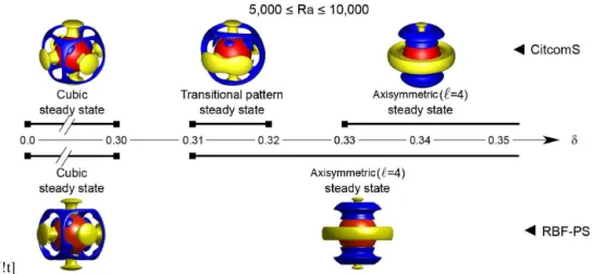
At low Rayleigh number, 5000≤Ra≤10 000, the cubic steady-state pattern is stable for both models up toδ=0.30.
In other words, the cubic pattern is maintained if the ratio of the spectral coefficient ofY44toY40is at least 1/2. This can be
seen in Fig. 2, where the isosurfaces of residual temperature (see caption for further details, as this is how 3-D convection will be illustrated in the paper) are plotted as a function ofδ.
Incrementing δ by 0.01, the RBF-PS model displays a clear transition between the cubic steady state and an order
ℓ=4 axisymmetric pattern. In contrast, CitcomS converges to a transitional steady-state pattern for 0.31≤δ≤0.32, in which the four plumes along the equator grow and merge to-gether two by two, but the process is not completed. This is never observed with the RBF-PS discretization (see Fig. 2). At higher values ofδ, CitcomS and the RBF-PS method con-verge to the same pattern. Thus, at the parameter value of destabilization (δ=0.30), the numerical discretization plays
an important role in what pattern emerges. Also, the transi-tion point at which the Y40 spherical harmonic mode
com-pletely dominates and theY44part of the initial condition no longer influences the final pattern of convection differs be-tween the two models.
Figure 3 shows the evolution of the volume-averaged tem-perature (< T >) for both models at Ra=7000. As just discussed, the figure illustrates that CitcomS converges to three different steady states, depending on the value ofδ. In
contrast, forδ >0.30, the figure shows that the RBF-PS
so-lution is attracted to theℓ=4 axisymmetric mode. In either case, the solution, once destabilized, transitions to patterns characterized by a higher< T >.
3.2 Sensitivity to amplitude perturbations in the initial condition at highRa
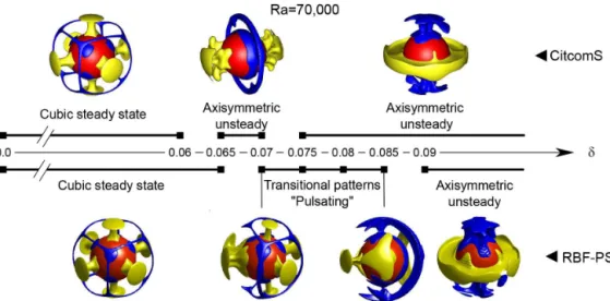
As would be expected, at higherRa, the cubic steady state is much more sensitive to small perturbations in the initial con-dition. ForRa=70 000, theY44mode of the initial condition was very slowly perturbed in increments of δ=5×10⁻³, as shown in Fig. 4. The cubic steady state is destabilized at δ≥0.065 for CitcomS and δ≥0.070 for the RBF-PS
method with different transitional patterns.
With CitcomS, the destabilization shows a transitional pat-tern between a cubic steady state to an unsteady axisymmet-ric pattern atδ=0.065 andδ=0.007, characterized by two diametrically opposed upwelling plumes in the equatorial re-gion with a great circle of downwelling that encompasses the polar regions. It develops via a two-by-two merging of up-welling plumes on the equator; initial upup-welling plumes at the poles are destabilized and migrate to the equatorial re-gion. The end state for perturbations ofδ≥0.75 is also an unsteady axisymmetric pattern. However, the pattern of con-vection has been completely rearranged, with upwelling now occurring in the polar regions and downwelling in the equa-torial region, yielding a strong dominance of an oscillating
ℓ=2 mode. The quasi-uniform oscillation of this end state can be seen in the time traces of the outerN uand
volume-averaged root-mean-square (rms) velocity in Fig. 5, where the region fort≥0.2 has been enlarged for better viewing.
With the RBF-PS model, the cubic steady state also even-tually evolves into an unsteady axisymmetric pattern for
δ≥0.085, similar to that of the CitcomS as shown in Fig. 4. However, the transition between these two states is very dif-ferent than what was observed with the CitcomS model. For
δ=0.07, the cubic pattern is only partially destabilized. Two plumes on one side merge and begin to pulsate. Although this structure is unsteady, it stays stable with no other changes in the general pattern of convection observed. Atδ >0.075, the cubic geometry is fully destabilized and the model begins to converge to the unsteady axisymmetric pattern, seen for
δ >=0.09.
[!t]
Figure 2.Final convection patterns resulting from perturbations,δ, to the cubic initial condition as obtained with CitcomS (top row) and the RBF-PS method (bottom row). Diagram is valid for 5000≤Ra≤10 000. The isosurfaces show the residual temperatureδT=T (r, θ, λ)− hT (r)i, wherehT (r)iis the horizontally average temperature. Blue (downwelling – descending motion) and yellow (upwelling – ascending motion) isosurfaces are forδT equal to−0.15 and 0.15, respectively. The red solid sphere is the inner boundary.
0.32
0.30
0.28
0.26
0.24
0.22
0.200 0.2 0.4 0.6 0.8 1
time
ave
rag
e
temp
er
at
ure
δ=0 δ=0.1 δ=0.2 δ=0.3 δ=0.31 δ=0.32 δ=0.33 0.32
0.30
0.28
0.26
0.24
0.22
0.200 0.2 0.4 0.6 0.8 1
time
ave
rag
e
temp
er
at
ure
RBF-PS
a)
b)
CitcomS
Figure 3.Time trace of the volume-averaged temperature for the cubic initial conditions at Ra=7000 for 0≤δ≤0.33. CitcomS shows transition to three steady states, while RBF-PS shows only two. See Fig. 2 for the final pattern of convection associated with each model.
Ra >30 000. In all cases, using RBF-PS, the transition is not characterized by a single pattern, as in CitcomS, but by a pro-gressive transition as a function of the perturbation (δ).
Sur-prisingly, this transitional regime broadens for large Rayleigh numbers (see red shaded area withRa≥50 000), implying larger perturbations are required to fully diminish the influ-ence of theℓ=4 modes. These results clearly demonstrate how numerical discretization impacts pattern formation and its interpretation in simulations of 3-D convective flow.
4 Stability at higher orders of symmetry: a dodecahedral initial condition
In Busse (1975), a steady-state higher-order convection pat-tern corresponding to dodecahedral symmetry is predicted. Here, for the first time (to the authors’ knowledge), the sta-bility of this pattern for lowRais studied, with surprising results on how the numerical discretization scheme severely affects the interpretation of steady-state stability ranges. The initial condition is given by Eq. (6) with
TP(θ, λ)= "
Y60(θ, λ)+ r
14 11Y
5 6(θ, λ)
#
. (10)
Theθ−λ temperature dependence on a sphere is shown
in Fig. 7. It has 12 initial plumes of upwelling, forming the faces of a dodecahedron, where the strongest downwelling (in dark blue) occurs at the vertices of the pentagons.
Figure 4.Stability of the cubic steady state atRa=70 000 with CitcomS (up row) and the RBF-PS method (bottom row). The cubic steady-state pattern is destabilized forδ≥0.065 with CitcomS andδ≥0.07 with RBF-PS. The figure highlights transitional patterns between the two main geometries.
time
0.2 0.3 0.4 0.5 0.6
130 140 150 130 135 140 145
RBF-PS
CitcomS VRMS
VRM
S
0 0.1 0.2 0.3 0.4 0.5 0.6
time 0
600
500
400
300
200
100
RMS
Vel
ocit
y
b)
RBF-PS
CitcomS
6.2 7.0 6.4 6.6 6.8
6.6
Nu
o
Nu
o
0 0.1 0.2 0.3 0.4 0.5 0.6
time 30
0 25
20
15
10
5
O
ut
er
Nu
a) CitcomS withδ=0.08
RBF withδ=0.09
time
0.2 0.3 0.4 0.5 0.6
Figure 5.Time trace of(a)the outer Nusselt number and(b)the rms velocity for both models atRa=70 000 forRa=70 000 andδ=0.08 with CitcomS andδ=0.09 with RBF. Both methods converge to an unsteady oscillating axisymmetric pattern dominated by theℓ=2 mode (see Fig. 4).
for the RBF-PS model, plumes do not merge untilt=2.7.
Surprisingly, the final stable stationary state differs between the two numerical discretizations: RBF-PS converges to a tetrahedral pattern, dominated by aℓ=3 mode, while Cit-comS reaches the cubic pattern studied in the previous sec-tion. In order to reduce the possible effect of spatial dis-cretization error, mesh resolution in CitcomS was increased by a factor of 8 to 12×963and doubled in the RBF-PS to 51(r)×6561(θ, λ). The results are displayed in Fig. 8. The
P
er
tur
bat
io
n
(
δ
) Axisymmetric unsteady state
Ra=70000
5 10 20 30 40 50 60 70 80 90 100
0 0.1 0.2 0.3 0.4 0.5
Rayleigh number (x1000) Ra=20000
Ra=7000
Cubic steady state
Axisymmetric
( = 4) steady state CitcomS
RBF-PS
Figure 6. Stability domain of the cubic steady-state pattern as a function of the perturbation to the initial condition, δ, and the Rayleigh number. Shaded areas show the transitional domains for the CitcomS (blue) and RBF-PS (red) methods. Detailed patterns are presented in Fig. 2 for 5000≤Ra≤10 000 and Fig. 4 for Ra=70 000. For each model, the bottom curve is the maximumδ value for which it converges to the cubic steady state, while the top curve is the minimumδvalue which converges to an axisymmetric pattern (steady or unsteady). The black dotted line is the value of the Rayleigh number that marks the transition between theℓ=4 steady state and the unsteady state.
-0.4 -0.2 0 0.2 0.4 0.6 0.8
TP
Figure 7.θ−λtemperature dependence of the dodecahedral initial condition (Eq. 10).
For CitcomS, the mesh discretization shows a symmetri-cal effect. The shell is initially divided in 12 caps. Each cap is diametrically opposite to another one (Zhong et al., 2000). Thus during the transition, we can observe that destabiliza-tion occurs in symmetrical pairs with respect to the caps. As a result it is reasonable to presume that mesh discretization and the cap divisions influence the distribution of numer-ical errors and favor even modes. Under these conditions, CitcomS will not reproduce the tetrahedral or the five-cell
RBF-PS: 43x4096 RBF-PS: 51x6561 CitcomS: 12x48x48x48 CitcomS: 12x96x96x96
RM
S
V
elo
cit
y
time
0 1 2 3 4 5
0 10 20 30 40 50 45
35
25
15
5
0.5 1.5 2.5 3.5 4.5
Dodecahedron unsteady state
Tetrahedron steady state
Cubic steady state
Figure 8.Time trace of the rms velocity for both models atRa= 7000 for two different spatial resolutions.
pattern observed with the RBF method without adding an ad-ditional initial perturbation representing these odd modes.
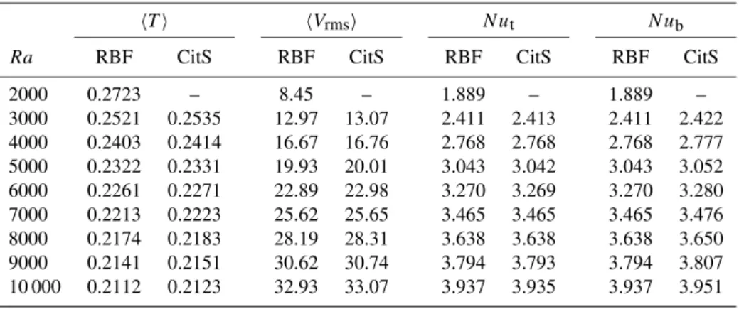
The stability of the dodecahedral steady-state solution for 2000≤Ra≤10 000 can also be seen in the time evolution of the volume-averaged rms velocity and the inner and outer Nusselt numbers as given in Fig. 9. In all cases of theRa,
the dodecahedral convection pattern is initially observed and stationary. This pattern is identical in both methods, whether one considers its geometry, the convergence of rms veloc-ity, average temperature, or Nusselt numbers before the tran-sition (Table 1). However, weakly unstable modes of lower spherical harmonic degree become excited and cause the so-lution to transition to a second steady state. When this transi-tion occurs in the time evolutransi-tion is clearly dependent on the model. For instance att=2, CitcomS has already reached a steady-state cubic pattern while RBF-PS is still in the weakly unstable steady-state dodecahedral pattern.
Ra = 7,000 Ra = 8,000 Ra = 9,000
Ra = 3,000 Ra =10,000
Ra = 2,000
RMS
Vel
ocit
y
0 1 2 3 4 5 6 7 8 9 0
10 20 30 40 50 60 70
time 0 1 2 3 4
0 10 20 50 60 70
RMS
Vel
ocit
y
time 30
40
0 1 2 3 4 5 6 7 8 9 time
8 7 6 5 4 3 2 9
1
O
ut
er
Nu
O
ut
er
Nu
0 1 2 3 4
time 8
7 6 5 4 3 2 9
1
0 1 2 3 4
time 4.5
1.0 4.0
3.5
3.0
2.5
2.0
1.5
Inne
rN
u
4.5
1.0 4.0
3.5
3.0
2.5
2.0
1.5
Inne
rN
u
0 1 2 3 4 5 6 7 8 9 time
Ra = 4,000 Ra = 5,000 Ra = 6,000 10
10
10 RBF-PS
RBF-PS
RBF-PS CitcomS
CitcomS CitcomS
Figure 9.Transition between steady states, as evidenced by both the RBF-PS and CitComS models, in thehVrmsi(top panels),N ui(middle
panels), andN uo(bottom panels) for the dodecahedral initial condition.
Table 1.Comparison between computational methods RBF and CitcomS for the dodecahedral stationary pattern at various Rayleigh number. For CitcomS and aRa=2000, the dodecahedral pattern does not satisfy stationarity to estimate parameters value.
hTi hVrmsi N ut N ub
Ra RBF CitS RBF CitS RBF CitS RBF CitS
2000 0.2723 – 8.45 – 1.889 – 1.889 –
3000 0.2521 0.2535 12.97 13.07 2.411 2.413 2.411 2.422
4000 0.2403 0.2414 16.67 16.76 2.768 2.768 2.768 2.777
5000 0.2322 0.2331 19.93 20.01 3.043 3.042 3.043 3.052
6000 0.2261 0.2271 22.89 22.98 3.270 3.269 3.270 3.280
7000 0.2213 0.2223 25.62 25.65 3.465 3.465 3.465 3.476
8000 0.2174 0.2183 28.19 28.31 3.638 3.638 3.638 3.650
9000 0.2141 0.2151 30.62 30.74 3.794 3.793 3.794 3.807
10 000 0.2112 0.2123 32.93 33.07 3.937 3.935 3.937 3.951
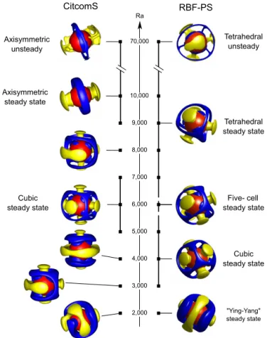
a newly observed five-cell pattern emerges as the end station-ary state in the RBF-PS model. It results from a mixed-mode interaction between the ℓ=3 andℓ=4 modes, as will be discussed in the next section. For 6000≤Ra≤10 000, the final pattern of convection for RBF-PS is the tetrahedral pat-tern observed in Fig. 8. In contrast, CitcomS transitions to
a stable steady-state axisymmetricℓ=2 pattern. ForRa >
RBF-PS
Cubic steady state Axisymmetric steady state
Cubic steady state
Tetrahedral steady state
2,000 3,000 4,000 5,000 6,000 7,000 8,000 9,000 10,000 70,000 Ra
Five-cell
steady state Axisymmetric
unsteady
CitcomS
"Ying-Yang" steady state
Tetrahedral unsteady
Figure 10.Transition of dodecahedral plume formation to different steady states for 2000≤Ra≤10 000 and to an unsteady state for 10 000< Ra≤70 000 with the RBF-PS method (right column) and CitcomS (left column).
5 A new convection mode: five cells
At 5750≤Ra≤6050 with RBF-PS method, the weakly un-stable dodecahedral pattern relaxed into a steady-state five-cell convection pattern. This structure is characterized by five upwelling plumes: two at the poles, each surrounded by a triangular region of downwelling, and three along the equa-tor, each surrounded by a square region of downwelling. The pattern appeared for a narrow range of Rayleigh numbers, between the cubic pattern at lower Rayleigh number and the tetrahedral pattern at higher Rayleigh number. This observa-tion along with the fact that the convective regions of de-scending motion are defined by both the vertices of a tri-angle in the polar regions (the case for the tetrahedral pat-tern) and those of a square in the equatorial regions (the case for the cubic pattern) leads us consider a mixed-mode inter-action between theℓ=3 and an ℓ=4 modes for an initial condition. Previous studies of mixed-mode patterns bifurcat-ing from spherically symmetric ones have been predicted in Busse and Riahi (1988) and numerically observed in Feudel et al. (2011). However, these studied reported a seven cell pattern resulting from an interaction of a ℓ=4 and ℓ=5
-0.4 -0.2 0 0.2 0.4 0.6
-0.4 -0.2 0 0.2 0.4 0.6
a)
b)
TP
TP
Figure 11.θ−λtemperature dependence of the five cells’ initial condition (Eq. 11) with(a)γ= 12and(b)γ=1110.
modes. In Chossat and Beltrame (2014), the authors investi-gatedℓ=3,4 mode interactions in a context compatible with
Rayleigh–Bénard convection without having highlighted the occurrence of a five-cell structure. Here, we focus on the for-mation of a steady-state five-cell pattern that is stable at large Rayleigh number,Ra=50 000, approximately 70 times the critical Rayleigh number (Rac=712, the onset of convec-tion).
Through numerical experimentation, we discovered that a combination ofY33andY40spherical harmonics will yield a five-cell pattern. However, in order to determine the volume-averaged spectral energies or variances between the two modes that yield the fastest stabilization in a five-cell steady-state pattern, a parameterγ on theY40mode is introduced. It will be varied slowly fromγ equals 0 to 1, in increments of
10−2. The initial condition is now given by Eq. (6) with
TP(θ, λ)= h
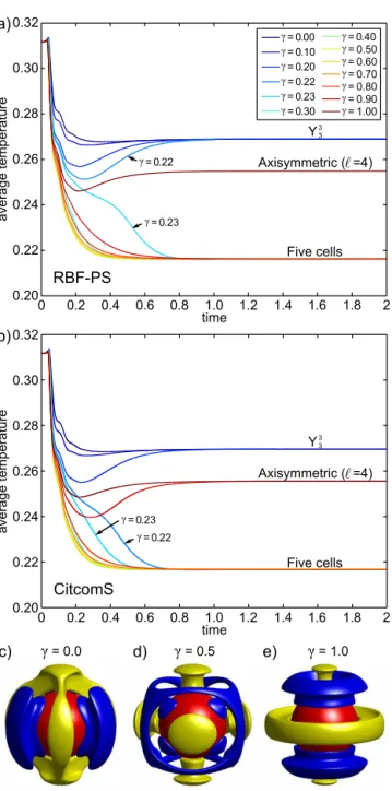
Y33(θ, λ)+γ Y40(θ, λ)i. (11) Figure 11 displays the initial conditions for two different values ofγ that will lead to two different steady states.
Five cells
γ= 0.0 γ= 1.0
averag
e
temper
at
ure
0.32
0.30
0.28
0.26
0.24
0.22
0.20
0 0.4 0.8 1.2 1.6 2
time
γ= 0.5
a)
c) d) e)
averag
e
temper
at
ure
0.32
0.30
0.28
0.26
0.24
0.22
0.20
0 0.4 0.8 1.2 1.6 2
time
b)
RBF-PS
CitcomS
0.2 0.6 1.0 1.4 1.8
0.2 0.6 1.0 1.4 1.8
γ= 0.00 γ= 0.10
γ= 0.40
γ= 0.30 γ= 0.22 γ= 0.20
γ= 0.50 γ= 0.60 γ= 0.70 γ= 0.80 γ= 0.90 γ= 1.00
γ= 0.22
Five cells Y3
3
Axisymmetric ( =4)
Y3 3
Axisymmetric ( =4)
γ= 0.22
γ= 0.23
γ= 0.23 γ= 0.23
Figure 12.Time traces of the evolution of the average temperature as a function of the parameter at Ra=7000 for(a)the RBF-PS model and(b)CitcomS.(c–e)show the final convection patterns for each of these models, with(c)γ=0,(d)γ=0.5, and(e)γ=1.
the value ofγ, the model converges to three distinct steady states. Forγ ≤0.20, theℓ=4 mode has no influence and the models converge to a steady state defined by theY33 spheri-cal harmonic mode. This pattern is similar to that found in Busse and Riahi (1988), except that there is a merging of the ascending motion in the polar regions. The steady-state five-cell pattern shown in Fig. 12d manifests itself in both models for 0.2≤γ <0.3, with the fastest stabilization to this state forγ=0.5. As a result, this is what will be used when
a) Ra=7000 b) Ra=10000 c) Ra=20000
d) Ra=30000 e) Ra=40000 f) Ra=50000
Figure 13.Stability of steady-state five-cell convection pattern as a function of the Rayleigh, displayed by the residual temperature for γ=0.5 (a) Ra=7×10³, (b) 104, (c) 2×10⁴, (d) 3×10⁴, (e)4×10⁴and(f)5×10⁴.
observing the stability of the five-cell pattern as a function of Rayleigh number. With the RBF-PS model, once the volume-averaged spectral energies between the two modes are equal (i.e.,γ=1), the flow reverts to an axisymmetric steady state, dominated by theℓ=4 mode. With the CitcomS model, the ratio of the modes only have to be within 10 % of one another (i.e.,γ=0.9) for this to occur. Lastly, Fig. 13 shows that this convection pattern is not only steady but stable with respect to perturbing the Rayleigh number for values at least up to
Ra=50 000, 70 times the critical Rayleigh number. Both models obtained this result. Also, as the Rayleigh number increases, the boundary layer thickness decreases, as would be expected with increased convection.
6 Conclusions
In time-dependent fully nonlinear systems, when numerical simulations are performed, a great variety of complex spa-tiotemporal regimes can be observed depending on parameter values. However, what this paper has illustrated is that what patterns are actually observed and at which parameter values they manifest themselves is definitely impacted by the nu-merical discretization used. Since computation has become a third arm of physical understanding, along with experimenta-tion and analysis, it is important to highlight this fact so that a discretization scheme is not blindly applied just because it is commonly used, as in the case of spherical harmonics.
at low Rayleigh number were more similar between the mod-els, both destabilizing when the contribution of the nonax-isymmetricℓ=4 spherical harmonic mode in the initial con-dition fell below 50 %. However, CitcomS showed a transi-tion to three steady states as this mode was perturbed, while RBF-PS went directly to the ℓ=4 axisymmetric mode. At higher Rayleigh number, the difference in the transitional states manifested between the two models was more drastic. The effect of the numerical discretization on pattern for-mation at higher orders of symmetry, such as dodecahedral symmetry where the initial condition is defined by a com-bination of ℓ=6 spherical harmonic modes, was of even greater interest. Although deemed a stable state by Busse (1975) for Rayleigh numbers near the onset of convection (Rac=712), it was shown to be unstable (after a long com-putational period – equivalent to 25 times the age of the Earth) for a Rayleigh number of just 2.5 times Rac at ex-tremely high resolutions for both models. However, regard-less of the Rayleigh number, the convection evolved com-pletely differently for each model, with the end steady state also being very different. For example, at Ra=7000, the RBF-PS model evolved into a tetrahedral symmetry, and Cit-comS into a cubic symmetry.
Another outcome of differences in numerical discretiza-tion can be the discovery of a stable convecdiscretiza-tion pattern (with regard to perturbations in the Rayleigh number) that does not seem to have been highlighted in the literature. In study-ing the dodecahedral convection pattern, in a narrow range of the Rayleigh number, the RBF-PS model stabilized to a five-cell steady-state pattern that was never seen in the Cit-comS model regardless of the Rayleigh number. This led the authors to investigate its formation, discovering that it is a strongly stable steady-state pattern of convection up to
Ra=50 000. Both models agreed that it forms by the inter-action of theY33andY40modes.
As a general observation, both methods show a good match in the cubic and five-cell steady-state patterns, and even for the stationary dodecahedral pattern before the tran-sition. However, the above in-depth computational study strongly illustrates how numerical discretization can impact both the resulting patterns of convection and the transitional states that occur. This is particularly true when scientists have to rely on such simulations in cases of strongly non-linear systems with over a million unknowns. In such cases, eigenvalue stability analysis is simply not an option. Further-more, we hope to have shed some light on cases of higher-order symmetry (such as the dodecahedral case), as well as nonsymmetric cases such as the five-cell pattern discussed. Although these patterns of convection are not expected to be found in the Earth, they can further aid the verification, validation and comparison of new numerical methods, al-gorithms, and codes, as applied to mantle convection in the Earth and other terrestrial planets. We also hope that this pa-per will stimulate further investigation into how the type and
order of numerical discretization affects pattern formation in the context of benchmarking community codes.
Acknowledgements. Pierre-Andre Arrial and Louise H. Kellogg
were supported by National Science Foundation (NSF) grant DMS-0934317. NCAR is supported by the NSF. Natasha Flyer was supported by NSF grant DMS-094581 and Grady Wright was supported by NSF grant DMS-0934330.
Edited by: L. Gross
References
Bercovici, D., Schubert, G., Glatzmaier, G. A., and Zebib, A.: Three-dimensional thermal convection in a spherical shell, J. Fluid Mech., 206, 75–104, doi:10.1017/S0022112089002235, 1989.
Bercovici, D., Schubert, G., and Glatzmaier, G. A.: Modal growth and coupling in 3-Dimensional spherical con-vection, Geophys. Astrophys. Fluid Dyn., 61, 149–159, doi:10.1080/03091929108229041, 1991.
Brooks, A. N.: A Petrov-Galerkin Finite Element Formulation for Convection Dominated Flows, Ph.D. thesis, Cali. Inst. of Tech-nol., Pasadena, 1981.
Busse, F. H.: Patterns of Convection in Spherical Shells, J. Fluid Mech., 72, 67–85, doi:10.1017/S0022112075002947, 1975. Busse, F. H. and Riahi, N.: Patterns of Convection in
Spherical Shells 2., J. Fluid Mech., 123, 283–301, doi:10.1017/S0022112082003061, 1982.
Busse, F. H. and Riahi, N.: Mixed-mode patterns of bifurcations from spherically symmetric basic states, Nonlinearity, 1, 379, doi:10.1088/0951-7715/1/2/004, 1988.
Choblet, G., ˇCadek, O., Couturier, F., and Dumoulin, C.: ÖDIPUS: a new tool to study the dynamics of planetary interiors, Geophys. J. Int., 170, 9–30, doi:10.1111/j.1365-246X.2007.03419.x, 2007. Chossat, P. and Beltrame, P.: Onset of intermittent octahedral pat-terns in spherical Bénard convection, arXiv:0912.3709, 40 pp., 2014.
Elman, H., Meerbergen, K., Spence, A., and Wu, M.: Lyapunov In-verse Iteration for Identifying Hopf Bifurcations in Models of Incompressible Flow, SIAM J. Sci. Comput., 34, A1584–A1606, doi:10.1137/110827600, 2012.
Feudel, F., Bergemann, K., Tuckerman, L., Egbers, C., Fut-terer, B., Gellert, M., and Hollerbach, R.: Convection pat-terns in a spherical fluid shell, Phys. Rew. E, 83, 046304, doi:10.1103/PhysRevE.83.046304, 2011.
Flyer, N. and Fornberg, B.: Radial basis functions: Developments and applications to planetary scale flows, Comput. Fluids, 46, 23–32, doi:10.1016/j.compfluid.2010.08.005, 2011.
Flyer, N. and Wright, G. B.: Transport schemes on a sphere us-ing radial basis functions, J. Comput. Phys., 226, 1059–1084, doi:10.1016/j.jcp.2007.05.009, 2007.
Flyer, N. and Wright, G. B.: A radial basis function method for the shallow water equations on a sphere, Proc. Roy. Soc. A, 465, 1949–1976, doi:10.1098/rspa.2009.0033, 2009.
Shallow water simulations on a sphere, J. Comput. Phys, 231, 4078–4095, 2012.
Fornberg, B. and Piret, C.: A stable algorithm for flat radial basis functions on a sphere, SIAM J. Sci. Comput., 30, 60–80, 2007. Fornberg, B. and Piret, C.: On choosing a radial basis function and
a shape parameter when solving a convective PDE on a sphere, J. Comput. Phys., 227, 2758–2780, doi:10.1016/j.jcp.2007.11.016, 2008.
Kameyama, M. C., Kageyama, A., and Sato, T.: Multigrid-based simulation code for mantle convection in spherical shell using Yin-Yang grid, Phys. Earth Planet. Interiors, 171, 19–32, 2008. Machetel, P., Rabinowicz, M., and Bernardet, P.: Three-dimensional
convection in spherical shells, Geophys. Astrophys. Fluid Dyn., 37, 57–84, doi:10.1080/03091928608210091, 1986.
Meerbergen, K. and Spence, A.: Inverse Iteration for Purely Imag-inary Eigenvalues with Application to the Detection of Hopf Bifurcations in Large-Scale Problems, SIAM J. Matrix Analy. Appl., 31, 1982–1999, doi:10.1137/080742890, 2010.
Moresi, L.-N. and Solomatov, V. S.: Numerical investigation of 2D convection with extremely large viscosity variations, Phys. Flu-ids, 7, 2154–2162, doi:10.1063/1.868465, 1995.
Moresi, L. N., Zhong, S., and Gurnis, M.: The accuracy of fi-nite element solutions of Stoke’s flow with strongly varying viscosity, Phys. Earth Plan. Int., 97, 83–94, doi:10.1016/0031-9201(96)03163-9, 1996.
Ramage, A. and Wathen, A. J.: Iterative solution techniques for the stokes and Navier-Stokes equations, Int. J. Numer. Methods Flu-ids, 19, 67–83, doi:10.1002/fld.1650190106, 1994.
Ratcliff, J. and Schubert, G.: Steady tetrahedral and cu-bic patterns of spherical shell convection with temperature-dependent viscosity, J. Geophys. Res., 101, 25473–25484, doi:10.1029/96JB02097, 1996.
Stemmer, K., Harder, H., and Hansen, U.: A new method to simulate convection with strongly temperature- and pressure-dependent viscosity in a spherical shell: Applications to the Earth’s mantle, Phys. Earth Plan. Int., 157, 223–249, doi:10.1016/j.pepi.2006.04.007, 2006.
Tan, E., Choi, E., Thoutireddy, P., Gurnis, M., and Aivazis, M.: GeoFramework: Coupling multiple models of mantle convec-tion within a computaconvec-tional framework, Geochem. Geophys. Geosyst., 7, Q06001, doi:10.1029/2005GC001155, 2006. Womersley, R. S. and Sloan, I. H.: Interpolation and Cubature on
the Sphere, Website, http://web.maths.unsw.edu.au/~rsw/Sphere/ (last access: 24 March 2014), 2003/2007.
Wright, G. N., Flyer, N., and Yuen, D.: A hybrid radial basis function–pseudospectral method for thermal convection in a 3-D spherical shell, Geochem. Geophys. Geosyst., 11, Q07003, doi:10.1029/2009gc002985, 2010.
Yoshida, M. and Kageyama, A.: Application of the Yin-Yang grid to a thermal convection of a Boussinesq fluid with infinite Prandtl number in a three-dimensional spherical shell, Geophys. Res. Lett., 31, L12609, doi:10.1029/2004GL019970, 2004.
Young, R.: Finite-amplitude thermal convection in a spherical shell, J. Fluid Mech., 63, 695–721, 1974.
Zebib, A., Schubert, G., and Straus, J. M.: Infinite Prandtl number thermal convection in a spherical shell, J. Fluid Mech., 23, 257– 277, doi:10.1017/S0022112080002558, 1980.
Zebib, A., Schubert, G., Dein, J. L., and Paliwal, R. C.: Charac-ter and stability of axisymmetric thermal convection in spheres and spherical shells, Geophys. Astrophys. Fluid Dyn., 23, 1–42, doi:10.1080/03091928308209038, 1983.
Zhong, S., Zuber, M. T., Moresi, L., and Gurnis, M.: Role of temperature-dependent viscosity and surface plates in spheri-cal shell models of mantle convection, J. Geophys. Res., 105, 11063–11082, doi:10.1029/2000JB900003, 2000.