A robust deep convolutional neural network model for text categorization

(1)

Universidade Federal de Minas Gerais

Instituto de Ciências Exatas

Programa de Pós-Graduação em Ciência da Computação

A ROBUST DEEP CONVOLUTIONAL NEURAL

NETWORK MODEL FOR TEXT CATEGORIZATION

Edgard de Freitas Júnior

VOLUME I

(2)

(3)

A ROBUST DEEP CONVOLUTIONAL NEURAL

(4)

(5)

EDGARD DE FREITAS JÚNIOR

A ROBUST DEEP CONVOLUTIONAL NEURAL

NETWORK MODEL FOR TEXT CATEGORIZATION

Dissertation presented to the Graduate Program in Computer Science of the Universidade Federal de Minas Gerais in partial fulfillment of the requirements for the degree of Master in Computer Science.

A

DVISOR

:

A

DRIANO

A

LONSO

V

ELOSO

Belo Horizonte

(6)

Freitas Júnior, Edgard de.

F866r A robust deep convolutional neural network model for text categorization. / Edgard de Freitas Júnior. Belo Horizonte, 2016.

xxv, 157f.: il.; 29 cm.

Dissertação (mestrado) - Universidade Federal de Minas Gerais – Departamento de Ciência da Computação.

Orientador: Adriano Alonso Veloso

1. Computação – Teses. 2. Aprendizado do computador – Teses. 3. Processamento da linguagem natural (Computação) – Teses. I. Orientador. II. Título.

CDU 519.6*82 (043)

(7)

(8)

(9)

v

Acknowledgments

I would like to thank my sister Anna Lee for her support and exemplary life trajectory that

inspired my decision on taking this challenge.

This work would not have been possible without the patience and support of my

girlfriend Denise and her family.

I would also like to thank my friends Andréia Martinez, Salomão Fraga and Paulo

Fernando for their encouragement and support that kept me going along the way.

I would like to express my gratitude to Prof. Alfredo Loureiro and Prof. Marcos André

Gonçalves for their recommendation letters and confidence.

I specially thank my longtime friend Prof. Wagner Meira for his support and advices.

My sincere thanks to Prof. Renato Ferreira and NVIDIA Corporation for the donation

of the K40 GPU, without which would not been possible to run all the experiments.

Thanks to Prof. Marco Cristo for the opportunity to participate on a deep learning

course taught by LISA researches at UFAM.

I wish to specially thank my advisor, Prof. Adriano Veloso, for his patience, optimism

and availability to participate in long discussions about deep learning and philosophy

matters.

I would also like to thank all the students from the machine learning group at UFMG

(10)

(11)

vii

“Colorless green ideas sleep furiously.”

(12)

(13)

ix

Resumo

Categorização de textos é uma das tarefas mais importantes nas aplicações do domínio do

Processamento de Linguagem Natural (PLN), a qual consiste em associar automaticamente

categorias pré-definidas a documentos escritos em linguagem natural. Técnicas tradicionais

de aprendizado de máquina utilizam características elaboradas manualmente para a

construção dos modelos, tais como, n-gramas, palavras de negação, sinais de pontuação,

símbolos representando emoções, palavras alongadas e dicionários léxicos. Esta abordagem,

chamada de engenharia de características, além de requerer um trabalho árduo, resulta

geralmente em modelos que apresentam uma performance ruim em tarefas para as quais não

foram especificamente criados.

Neste trabalho, propomos um modelo robusto baseado em uma Rede Neural de

Convolução (RNC) profunda para aprendizado chamado de PLN profundo. Nosso modelo

utiliza uma abordagem composicional, na qual o projeto da arquitetura da RNC profunda

induz a criação de uma representação hierárquica para o texto através da descoberta de

representações intermediárias para as palavras e sentenças do texto. As representações

iniciais para as palavras, chamadas de incorporação de palavras, são obtidas de um modelo

de linguagem neural treinado previamente de forma não supervisionada, as quais são

ajustadas para o contexto da tarefa para a qual o modelo está sendo treinado.

O nosso modelo foi avaliado em tarefas de categorização de textos comparando sua

acurácia com os resultados publicados para alguns modelos tradicionais e de aprendizado

profundo utilizando seis conjuntos de dados de larga escala. Os resultados mostram que

nosso modelo é robusto no sentido de que, mesmo quando nós utilizamos os mesmos

parâmetros globais, ele supera a acurácia dos modelos considerados estados da arte em

diferentes tarefas de categorização de textos. Os resultados também mostram que a utilização

de um dicionário de sinônimos semânticos juntamente com as representações iniciais de

palavras ajuda na generalização das representações aprendidas pelo modelo, aumentando sua

acurácia.

(14)

(15)

xi

Abstract

Text categorization is the task of automatically assigning pre-defined categories to

documents written in natural languages and it is one of the most important tasks in Natural

Language Processing (NLP) domain applications. Traditional machine learning techniques

rely on handcrafted features such as ngrams, negation words, punctuation, emoticons, stop

words, elongated words and lexicons to build their models. This approach, called feature

engineering, in addition to being labor intensive, results in models that, in general, present

poor performance on tasks for what they have not been specifically tailored.

In this work, we propose a robust deep learning Convolutional Neural Network (CNN)

model named Deep NLP. Our model adopts a compositional approach, in which the design

of the deep CNN architecture induces the creation of a hierarchical representation for the

text, through the extraction of intermediate representations for the words and sentences of

the text. The initial word representations, called word embeddings, are obtained from a

pre-trained unsupervised neural language model and they are adjusted for the context of the task

that the model is being trained.

We evaluated our model comparing its accuracy against the results reported by some

traditional and deep learning models in text categorization tasks using six large-scale data

sets. The results show that our model is robust in the sense that, even when we use the same

hyperparameters, it surpasses the accuracy of the state-of-the-art models in different text

categorization tasks. The results also show that the use of a semantic synonyms dictionary

together with the word embeddings helps to generalize the representations learned by the

model increasing its accuracy.

(16)

(17)

xiii

List of Figures

Figure 2.1. Neuron model projected over a typical neuron cell. ... 9

Figure 2.2. Steps of the backpropagation algorithm. ... 11

Figure 2.3. The six layers of the human neocortex... 12

Figure 2.4. Representations learned by layers make data separable... 13

Figure 2.5. Effect of the number of parameters on the performance of models with different depths. ... 14

Figure 2.6. Evolution of GPUs and NNs over time. ... 15

Figure 2.7. Evolution of data sets size over time. ... 16

Figure 2.8. 2D convolution operation. ... 17

Figure 2.9. Patterns learned by the layers of a deep CNN. ... 17

Figure 2.10. 1D convolution sparse connectivity and parameters sharing. ... 18

Figure 2.11. A typical CNN layer. ... 19

Figure 2.12. Architectures of the CBOW and Skip-gram neural language models. ... 21

Figure 2.13. Algebraic operations on word vectors. ... 21

Figure 4.1. Model data flow. ... 28

Figure 4.2. Deep NLP model architecture. ... 31

Figure 5.1. Main components of a Torch7 NN package module... 35

Figure 5.2. Lua code fragment of the deep CNN model implementation. ... 36

Figure 5.3. Execution log excerpt of the deep CNN model... 37

Figure 5.4. Input text decoding through the lookup table forward method. ... 38

Figure 5.5. Temporal convolution over the decoded input text. ... 39

Figure 5.6. Plot of the threshold function and its derivative. ... 40

Figure 5.7. Detailed diagram of our deep CNN architecture. ... 43

Figure 5.8. Detailed diagram of our deep CNN architecture. ... 44

(18)

xiv

(19)

xv

List of Tables

Table 6.1. Characteristics of the large-scale data sets used in the experiments... 47

Table 6.2. AG's news data set samples. ... 48

Table 6.3. AG's news documents statistics. ... 49

Table 6.4. DBPedia ontology data set samples. ... 50

Table 6.5. DBPedia ontology documents statistics. ... 51

Table 6.6. Yelp reviews polarity data set samples. ... 51

Table 6.7. Yelp reviews polarity documents statistics. ... 52

Table 6.8. Yelp reviews full star data set samples. ... 52

Table 6.9. Yelp reviews full star documents statistics. ... 53

Table 6.10. Yahoo! Answers data set samples. ... 54

Table 6.11. Yahoo! Answers documents statistics. ... 55

Table 6.12. Amazon reviews polarity data set samples. ... 56

Table 6.13. Amazon reviews polarity documents statistics. ... 56

Table 6.14. Values of the model hyperparameters used in the experiments... 57

Table 6.15. Minimum vocable frequencies used in experiments. ... 58

Table 6.16. Vocabulary size and number of parameters of the model. ... 58

Table 6.17. Amazon reviews polarity training data set size experiment. ... 59

Table 6.18. Computer hardware specification. ... 60

Table 7.1. Accuracy results summary. ... 62

Table 7.2. Training data sets comparison. ... 63

Table 7.3. Vocabulary generation and text encoding statistics using WordNet. ... 63

(20)

(21)

xvii

List of Acronyms

1D One-dimensional

2D Two-dimensional

ANN Artificial Neural Network

BoW Bag of Words

CBOW Continuous Bag-of-Words

CNN Convolutional Neural Network

DBN Deep Belief Network

DCNN Dynamic Convolutional Neural Network

GPU Graphical Processing Unit

ILSVRC ImageNet Large-Scale Visual Recognition Challenge

LSTM Long Short Term Memory

NLL Negative Log-Likelihood

NLP Natural Language Processing

NLTK Natural Language Toolkit

NN Neural Network

POS Poverty of the Stimulus

RecNN Recursive Neural Network

ReLU Rectified Linear Unit

RNN Recurrent Neural Network

SGD Stochastic Gradient Descent

(22)

(23)

xix

Introduction

Text categorization is one of the most important tasks in Natural Language Processing

(NLP). Text categorization is the task of automatically assigning pre-defined categories to

documents written in natural languages. Text categorization can be used for, among others,

classifying a document in a set of topics, rating a product review written by a costumer or

associating a sentiment with a text posted by a user [Manning & Schütze, 1999] [de Oliveira

Jr., et al., 2014] [Veloso, Jr., Cristo, Gonçalves, & Zaki, 2006].

Traditional machine learning techniques used to build models for text categorization

rely on handcrafted features to succeed. Features such as ngrams, negation words, stop

words, punctuation, emoticons, elongated words and lexicons are carefully chosen by a

domain specialist for a specific task. This approach leads to models tailored for a specific

context and seldom achieve good performance in different tasks. This approach is called

feature engineering [Bottou, et al., 2011].

1.1 Deep Learning Models

The deep learning paradigm adopts a different approach to find the model features. The

models built using the deep learning approach learn not only the parameters of the features

but also the features themselves for a given task. This approach, called feature learning, leads

to more general models that achieve good performance in different tasks and domains . In

this scenario, the model specialist has to fine-tune the model hyperparameters for the given

(28)

2 CHAPTER 1. INTRODUCTION

Despite the good performance achieved by some traditional machine learning NLP

techniques as Bag of Words (BoW) in text categorization tasks such as topic identification,

these models present poor performance in tasks where the semantic of the text is sensitive to

the word positions. For example, a BoW model will give the same value for the expressions

“know a little bit about everything” and “know everything about a little bit”. Both

expressions have exactly the same words, but have different meanings. The first one

designates a generalist and the second one designates a specialist. To be able to capture the

semantic of a sentence, a model has to take into account the word positions in the sentence.

There are different deep learning models suited for specific application domains. The

Recursive Neural Network (RecNN) model is claimed to be well suited for NLP applications

because of its hierarchical structure. The weakness of this type of model is its dependency

on an external syntactic parse tree. This restriction limits the learning of semantic relations

between words to syntactically dictated phrases. Extended models based on RecNN achieved

the state of the art in some NLP tasks using specific data sets [Socher, et al., 2013].

The Recurrent Neural Network (RNN) model is a special case of RecNN that is suited

for modeling sequential data. Despite its power in representing sequential structures, it is

seldom being used for NLP tasks such as text categorization because of its difficulty in

learning long-term dependencies. This limitation is due to the exploding and vanishing

gradients problems that occur in the training phase [Pascanu, Mikolov, & Bengio, 2013].

To overcome the exploding and vanishing gradients problems, a type of RNN

architecture called Long Short Term Memory (LSTM) has been used with success in some

application domains [Zaremba, Sutskever, & Vinyals, 2014].

1.2 Convolutional Neural Network Models

Two-dimensional (2D) Convolutional Neural Network (CNN) models have been

successfully applied in computer vision domain problems for some time [LeCun, Bottou,

Bengio, & Haffner, 1998]. More recently, the remarkable results achieved by deep CNN on

image classification challenges got the state of the art to a new level and promoted the

(29)

CHAPTER 1. INTRODUCTION 3

It has been showed that deep CNN models are able not only to discover the features of

the data, but also they are able to learn a hierarchical representation for the data through the

discovered features. The revealed features have desirable properties such as

compositionality, increasing invariance and class discrimination as they ascend the network

layers [Zeiler & Fergus, 2013].

One-dimensional (1D) CNN models like Time-Delay Neural Networks (TDNN) have

been successfully used for some time in speech recognition applications such as phoneme

recognition [Waibel, Hanazawa, Hinton, Shikano, & Lang, 1989]. More recently, deep

1D-CNN models have been used in NLP tasks like language modeling [Bottou, et al., 2011].

1.3 Data Representation

A central problem present in all NLP applications is how to represent the input text. Some

models view the input text as a stream of characters [Zhang, Zhao, & LeCun, 2015]. Other

models deal with the input text as a sequence of phonemes [dos Santos & Gatti, 2014]. Most

models make the natural choice of viewing the input text as a sequence of words. In these

models, the problem is how to represent a word. The simplest way is to associate with each

vocable present in the text a unique id and use a lookup table to encode the text’s words.

Each id is represented as a vector that has the size of the vocabulary and only the bit that

identifies the vocable is set to one. That is why this type of word representation is called

one-hot.

The problem with the one-hot representation is the dimensionality of the word vectors.

For example, in a dataset with 30K vocables, each word in the text will be represented by a

vector of size 30K. Despite of this limitation, some models using one-hot representation have

achieved remarkable results in text categorization tasks [Johnson & Zhang, 2015].

A more sophisticated way of word representation is called word embedding. This type

of representation tries to create a mapping from the symbolic representation of a word into

a lower dimensional vector space. In addition to effectively dealing with the problem of the

dimensionality, it has been shown that word embeddings are able to capture many semantic

(30)

Intuitively, in the context of deep learning models, the use of word embeddings makes

sense. Like humans do, the model learns a semantic representation of a word in some context

and it adjusts this representation for the specific context that it is being trained. The models

that make use of word embeddings are considered semi-supervised models because the

initial word representations are learned in an unsupervised way and they fit these

representations for a specific task through a supervised training.

1.4 Compositionality

Another central problem present in all NLP tasks is how much syntax is needed to extract

semantics. As we have already mentioned, the RecNN models depend on an external

syntactic parse tree to extract semantic from a text. The performance of these models

degrades on NLP tasks where the input text is written using an informal language style that

does not strictly follow syntactic rules.

Some models try to learn a representation in an unsupervised way not only for the

words but also for the whole paragraph. These models are suited for NLP tasks where there

is not data sets with enough labeled data. [Le & Mikolov, 2014]

Most of the deep CNN models used in NLP tasks convolves a set of filters over the

sequence of text words. They do not explicitly take into account the syntactic information of

text sentence units. They consider the whole text as a syntactic unit. These models are suited

for NLP tasks where the input text holds in one sentence. An example of this type of task is

sentiment classification of texts from a Twitter dataset [Kalchbrenner, Grefenstette, &

Blunsom, 2014].

In some NLP tasks, it seems to make sense to apply a compositional approach. These

models explicitly consider a text made up by sentence units that, in turn, are compounded

by words [Denil, Demiraj, Kalchbrenner, Blunsom, & de Freitas, 2014].

Analogously to an image made up by different classes of objects in the computer vision

domain, a text is made up by sentence units that can have different semantics. It was showed,

in the computer vision domain, that forcing information to pass through carefully chosen

(31)

the model [Hinton, Krizhevsky, & Wang, 2011]. This strategy helps on the generalization of

the representations learned by the model [Gülçehre & Bengio, 2013].

1.5 Depth

Another central question in the design of deep learning models is how deep a network must

be. There is a consensus that shallow models are not able to extract complex features of the

data but there is not a rule of thumb to determine how many layers suffice to extract the

required features for a specific task. In the computer vison domain, a deep CNN model that

achieved the state of the art in image classification tasks was implemented using 22 layers

[Szegedy, et al., 2014].

Another critical issue on the design of deep CNN models is the relationship between

the number of parameters and the depth of the model. In the specific case of NLP models,

the dimensionality of the data representation has a huge impact on the number of parameters

of the model.

1.6 Objectives of this Work

The objective of this work is to propose a robust deep CNN model for text categorization

tasks, named Deep NLP. The design of this model aims to overcome the limitations of other

models reported in the literature and to achieve a robustness in the sense that the model can

be used in different text categorization tasks without the need of tuning the model

hyperparameters. To achieve these objectives, we employ a series of deep learning concepts

and techniques. We adopt a semi-supervised approach where the initial vocable

representations are obtained from a pre-trained unsupervised neural language model publicly

available1 (Word2Vec). The vocable representations are adjusted to a specific task context

during the training phase. The model implements a compositional approach explicitly

creating intermediate representations for the sentences. The size of the input text is not

limited by the model. The model is made up of seven layers to extract complex features of

(32)

the input text. We make use of the WordNet corpus to find semantic synonyms for the

vocables not found in Word2Vec and for the text words not found in the generated

vocabulary [Miller, 1995].

1.7 Contributions of this Work

We evaluated our model comparing its accuracy against the results reported by deep learning

models in text categorization tasks [Zhang, Zhao, & LeCun, 2015]. The model was trained

without and with the use of the WordNet synonyms. We also made experiments to measure

how the data set size affects the accuracy and training time of our model.

The results show that our model is robust in the sense that, even when using the same

model hyperparameters, it can beat the state of the art models’ accuracy in different text

categorization tasks. The results also show that the use of the WordNet semantic synonyms

helps to generalize the representation learned by the model, thus increasing its accuracy. The

experiments made with the data set size show that our model beat the accuracy of the state

of the art model using only one third of the data set size.

Another contribution resultant from the design of the proposed architecture is that our

model do not impose any limit on the size of the input text. The implementation of our model

makes an efficient use of the massively parallel processing power of the GPU, which makes

it possible to train huge data sets in a shorter processing time.

1.8 Organization

The remaining part of this work is organized as follows. In Chapter 2, we introduce some

underlying concepts used in artificial neural networks and deep learning models. In Chapter

3, we present the related work that apply or develop similar concepts used in this dissertation.

In Chapter 4, we provide an in-depth description of the architecture of our model. In Chapter

5, we discuss the implementation details of our model. In Chapter 6, we describe the data

(33)

results of the experiments. In Chapter 8, we discuss the main contributions of this work. In

(34)

8

Chapter 2

Background

In this chapter, we present the underlying concepts necessaries for the understanding of this

work. We introduce some Artificial Neural Networks basic concepts, then we present some

principles discovered by the neural science that inspired the development of the

neurocomputing algorithms. Finally, we present an overview of the deep learning paradigm.

2.1 Neural Networks

The basic concepts used in the deep learning paradigm are inherited from the Artificial

Neural Networks (ANNs) models or Neural Networks (NNs) for short. The aim of the NNs

paradigm is to develop computer programs capable of solving abstract problems that are

hard to be described using formal rules, but are easily solved by human beings.

The development of the NNs paradigm started in the 1950s [McCulloch & Pitts, 1943]

[Rosenblatt, 1962]. The NNs models were inspired by the concepts and principles of the way

the human brain works, which was discovered by the neural science.

The human cortex can be viewed as a complex network whose nodes are neurons. Each

neuron receives input signals from other neurons through its dendrites. The neurons

connections are established through the synapses. The strength of the input signals is

determined by the stimulus received. The input signals are combined inside the neuron to

create an output signal. The output signal is transmitted to other neurons through the axon if

its amplitude is greater than a pre-determined value called action potential. The output signal

is called a spike. It is estimated that the human cortex has 10 billion of neurons and 60 trillion

(35)

CHAPTER 2. BACKGROUND 9

At the cell level, the human behavior adaptability or learning mechanism can be

explained by the plasticity hypothesis. The stimulus received from the environment and the

output produced by the network cause permanent changes on the neurons connections.

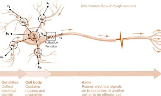
Figure 2.1 shows a node of a feedforward NN model projected over a schematic view of a

typical neuron.

In Haykin [1999], the author defines an ANN as a massively parallel distributed system

made up of simple processing units, which has a natural propensity for storing experimental

knowledge. An ANN resembles the human brain in that the knowledge is acquired by the

network from its environment through a learning process and the strength of neuron

connections, known as synaptic weights, are used to store the acquired knowledge.

In the context of ANNs, learning is the process by which the synaptic weights, or

network parameters, are adjusted through a process of stimulation known as training. The

type of learning is determined by the way the parameters changes take place. There are many

types of learning mechanisms. In ANNs, the most used learning mechanism is the

error-correction algorithm.

The error-correction learning algorithm compares the network output with a target

value through an objective or cost function. The cost function associates the network

parameters with a measure of the error produced by the network output. In feedforward NNs,

the most used error-correction learning algorithm is the backpropagation.

(36)

10 CHAPTER 2. BACKGROUND

Backpropagation is about understanding how adjusting the weights and biases in a

network changes the error given by the cost function. Because the cost function depends on

the network output value, which in turn is a function of the output layer activation function

that depends on the previous layers weights and bias and so on, we can recursively use the

chain rule to calculate the gradient of the cost function with respect to the network

parameters. This way, we know how the changes on each network parameter contribute to

the error measured by the cost function.

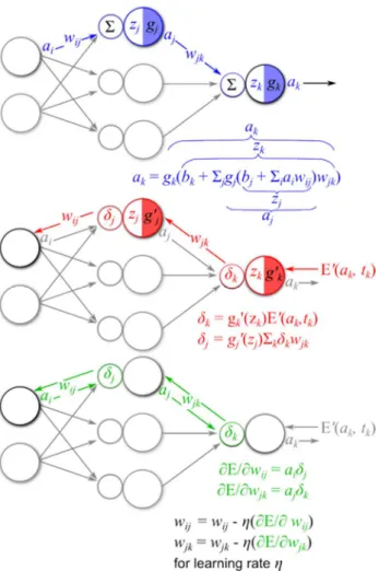
The backpropagation algorithm is executed in four steps. In the feedforward step, the

network output is calculated. In the error step, the cost function gradient of with respect to

the network output is calculated. In the backward step, the error is back propagated

calculating the gradient with respect to the previous layers outputs. In the update step, the

values of the network parameters are adjusted using some updating rule. In general, the

updating rule used is the gradient descent algorithm. The network parameters are subtracted

from its gradient multiplied by a constant. This constant is called the learning rate.

The backpropagation algorithm was originally introduced in the 1970s, but it became

popular only in 1986 after the publication of a paper in which the authors showed that the

speedup aroused from the use of the backpropagation algorithm made it possible to use NNs

to solve problems that had previously been insoluble [Rumelhart, Hinton, & Wilson, 1986].

What is clever about the backpropagation algorithm is that it enables us to compute all

the gradients partial derivatives simultaneously using just one forward pass through the

network, followed by one backward pass. Roughly speaking, the computational cost of the

backward pass is about the same as the forward pass.

Even in the late 1980s, people ran up against computational limits, especially when

attempting to use backpropagation to train deep NNs. The backpropagation algorithm is

based on common linear algebraic operations like vector additions and matrix

multiplications. In 2006, the improvement of the algorithms and the popularization of the

use of the GPUs for scientific computation made the use of the backpropagation algorithm

(37)

Figure 2.2 shows the steps of the backpropagation algorithm in a small segment of a

typical feedforward neural network.

2.2 Neocortex Deep Structure

Another concept used in ANNs inspired by the human cortex structure is the concept of

hierarchy. Humans organize their ideas and concepts hierarchically first learning simpler

concepts and then composing them to represent abstract concepts. It is believed that this

behavior is due to the physical structure of the human neocortex.

The human neocortex is organized into regions and the typical neocortex tissue is made

up by six layers of neurons cells. The lower layers, sixth and fifth, have a higher

concentration of neurons than the upper layers. They receive input signals from other cortex

(38)

regions and pass the extracted features to the upper layers, which in turn pass the information

to other neocortex regions.

Within the neocortex, the information flows serially from one region to another. For

example, the visual cortex is built by a sequence of regions, each of which contains a

representation of the input and the signals flow from one region to the next. Each level of

this feature hierarchy represents the input at a different abstraction level, with more abstract

features further up in the hierarchy, defined in terms of the lower-level ones [Kandel,

Schwartz, & Jessel, 2000].

The upper layers and regions also have feedback connections to the lower ones. For

many years, most scientists ignored these feedback connections. They are essential for the

brain to accomplish one of its most important functions, which is to make predictions.

Predictions requires a comparison between what is happening and what you expect to

happen. What is actually happening flows up in the hierarchy, and what you expect to happen

flows down [Hawkins & Blakeslee, 2004].

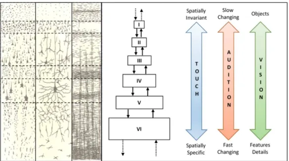
Figure 2.3 shows on the left a histological structure of the human neocortex tissue and

on the right a schematic representation of some sensory regions layers hierarchy. The

appearance of the histological structure depends on what was used to stain it. The Golgi stain

reveals the neuronal cell bodies and the dendritic trees. The Nissl method shows the cell

bodies and the proximal dendrites. The Weigert stain for myelinated fibers reveals the

pattern of axonal distribution [Kandel, Schwartz, & Jessel, 2000].

(39)

2.3 Deep Learning

2.3.1 Depth Matters

The deep learning paradigm can be characterized by the use of two strategies inspired by the

working of the human brain. The first strategy is the learning from experience, which was

already adopted in the ANNs. The second strategy is to understand the world in terms of a

deep hierarchy of concepts, with each concept defined in terms of its relation to simpler

concepts.

The approach of gathering knowledge from experience avoids the need to specify the

formal rules that allow the computer programs to solve abstract problems. The approach of

viewing an abstract problem as a hierarchy of concepts allows the computer programs to

learn complicated concepts by building them out of simpler ones.

The building of a hierarchy of concepts is induced by the deep architecture of layers.

The use of a deep architecture can be viewed as a kind of function factorization. The depth

of two layers may be enough to represent some families of functions with a given target

accuracy. Theoretical results showed that there are families of functions for which the

insufficient depth makes the number of parameters grows exponentially with the input size

[Bengio, 2009]. The Kolmogorov’s Mapping Neural Network Existence theorem assures

that an arbitrary continuous function, mapping values from an n-dimensional compact set to

the real numbers vector space, can be implemented by a feedforward neural network with at

least three layers of depth [Hecht-Nielsen, 1990].

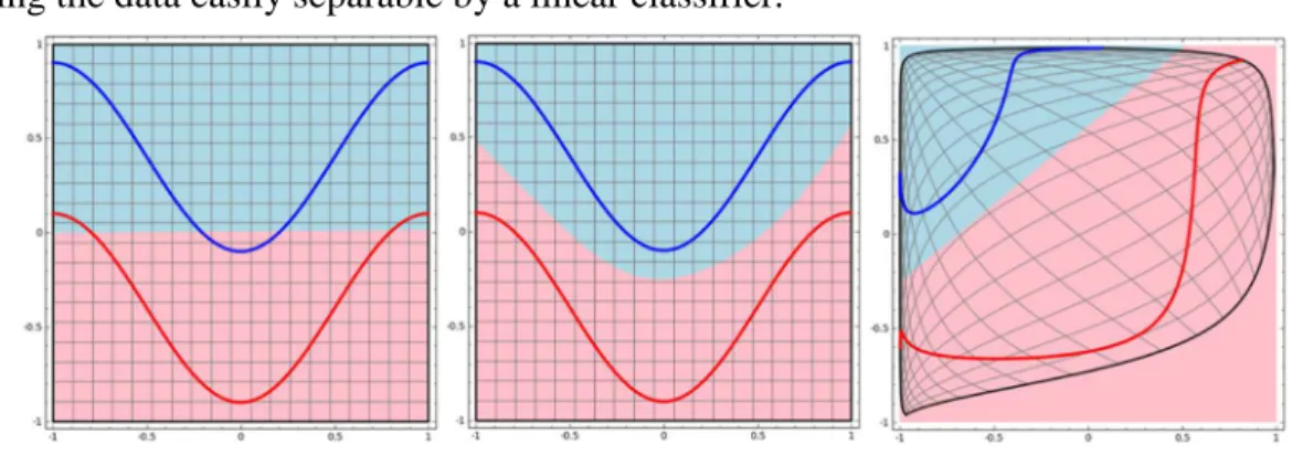
Figure 2.4 illustrates a classification problem of a two-class data set represented by

two curves. Each layer of the network transforms the data, creating a new representation and

making the data easily separable by a linear classifier.

(40)

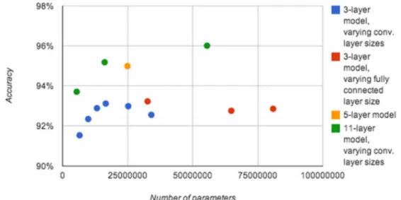
Deeper models tend to perform better not only because they are larger. Increasing the

number of parameters in models having less than three layers, called shallow models, does

not allow them to reach the same level of performance as deeper models. This is primarily

due to overfitting. Figure 2.5 presents a chart with the results of an experiment comparing

the number of parameters with the performance of models having different depths

[Goodfellow, Bulatov, Ibarz, Arnoud, & Shet, 2014].

It is clear that only the deepest models had their accuracy increased with the growth

on the number of parameters.

2.3.2 The Renascence

Until 2006, attempts of training a deep supervised feedforward neural network architecture

yielded worse results then shallow architectures. In Bengio et al. [2006], the authors

extended the pionner work done in Hinton et al. [2006,] showing that the initialization of

Deep Belief Networks (DBN) parameters with pre-trained unsupervised learned

representations values could improve its generalization. Since then, the development of new

algorithms and techniques made possible the implementation of deeper architecutes and the

adoption of the deep learning paradigm to solve problems in many domains [Bengio,

Learning Deep Architectures for AI., 2009].

Figure 2.5. Effect of the number of parameters on the performance of models

(41)

In 2012, a dramatic moment in the meteoric rise of deep learning came when a deep

CNN architecture won the ImageNet Large-Scale Visual Recognition Challenge (ILSVRC)

for the first time and by a wide margin, bringing down the state-of-the-art error rate from

26.1% to 15.3% [Krizhevsky, Sutskever, & Hinton, 2012]. Since then, these competitions

are consistently won by deep CNNs and the advances in deep learning have brought the

latest top-5 error rate in this contest down to3.6% [Goodfellow, Bengio, & Courville, 2016].

Two main facts, besides the development of new algorithms and techniques,

contributed to the recent success of the deep learning paradigm. The increase on the

massively parallel processing power of the GPUs for scientific computation made it possible

to implement deeper models having a huge number of parameters.

Figure 2.6 shows comparative charts between the processing power of the GPUs, on

the left, and the number of neurons of ANNs implemented over time on the right

[Goodfellow, Bengio, & Courville, 2016].

The other fact that contributed to the recent success of the deep learning paradigm is

the increase on the data sets size. In the 1980s and 1990s, machine learning became statistical

in nature and began to leverage larger data sets containing tens of thousands of examples

such as the MNIST data set. As the models become more complex, the number of parameters

increases and more data is required to train the model.

(42)

Figure 2.7 shows a chart of the data sets size over time [Goodfellow, Bengio, &

Courville, 2016].

2.3.3 CNN Architecture

There are many types of ANN architectures. Each architecture has been developed for a

specific task. The Convolutional Neural Network (CNN) architecture was developed for

computer vision tasks and it was inspired by the discoveries of the neurophysiologists about

how the mammalian vision system works [Hubel & Wiesel, 1959]. They observed how

neurons in the cat’s brain responded to images projected in precise locations on a screen in

front of the cat. Their great discovery was that neurons in the early visual system responded

most strongly to very specific patterns of light, such as precisely oriented bars, but responded

hardly at all to other patterns.

The visual cortex contains a complex arrangement of cells that are sensitive to small

sub-regions of the visual field, called a receptive field. The sub-regions are tiled to cover the

entire visual field. These cells act as local filters over the input space and are well suited to

exploit the strong spatially local correlation present in natural images. Simple cells respond

maximally to specific edge-like patterns within their receptive field. Complex cells have

larger receptive fields and are locally invariant to the exact position of the pattern.

The term convolutional comes from a mathematical operation called convolution.

Convolution is a specialized kind of linear operation. The convolution operation used in

ANNs does not correspond precisely to its definition in mathematics. Convolutional

(43)

networks are simply ANNs that use convolution in place of general matrix multiplication in

at least one of their layers [Goodfellow, Bengio, & Courville, 2016].

Figure 2.8 shows a schematic view of a 2D convolution operation as it is used in

ANNs. The small letters correspond to the values of each position of the input and of the

filter.

It has been showed that deep CNN models are able not only to discover the features of

the data, but also they are able to learn a hierarchical representation for the data through the

discovered features. The revealed features have desirable properties such as

compositionality, increasing invariance and class discrimination as they ascend the network

layers [Zeiler & Fergus, 2013]. Figure 2.9 shows the images generated by a visualization

technique called deconvolution. The images reveal the patterns learned by each layer of a

deep CNN. In the lower layers, the discovered patterns, like edges, correspond to small

regions of the image. In the upper layers, the discovered patterns, like objects, correspond to

larger regions of the image.

Figure 2.8. 2D convolution operation.

(44)

Another key consideration about the architecture design of ANNs is the connection

between the layers. Traditional ANN layers use a matrix multiplication to describe the

interaction between each layer. This means that every element of a layer is connected to

every element of the previous and next layers. CNNs have sparse connections. This is

accomplished by making the filter smaller than the input. For example, when processing an

image, the input image might have thousands or millions of pixels, but we can detect small,

meaningful features such as edges with filters that occupy only tens or hundreds of pixels.

This means that we need to store fewer parameters, which both reduces the memory

requirements of the model and improves its statistical eﬃciency. It also means that computing the output requires fewer operations. These improvements in e_ﬃciency are usually quite large.

Another strategy present in CNNs that helps reduce the memory requirements is the

parameter sharing. Parameter sharing refers to using the same parameter for more than one

function in a model. In a traditional ANN, each element of the weight matrix is used exactly

once when computing the output of a layer. It is multiplied by one element of the input and

then never revisited. As a synonym for parameter sharing, one can say that a network has

tied weights, because the value of the weight applied to one input is tied to the value of a

weight applied elsewhere. In a CNN, each element of the filter is used at every position of

the input. The parameter sharing used by the convolution operation means that rather than

learning a separate set of parameters for every location, the model learns only one set. CNNs

are thus dramatically more e_ﬃcient than dense matrix multiplication in terms of the memory requirements and statistical e_ﬃciency [Goodfellow, Bengio, & Courville, 2016]. Figure 2.10 shows a schematic view of the sparse connectivity and parameters sharing effects caused by

a 1D-convolution operation.

(45)

Figure 2.11 shows the three stages of a CNN typical layer. In the first stage, the layer

performs several convolutions in parallel to produce a set of linear activations. In the second

stage, each linear activation is run through a nonlinear activation function, such as the

rectified linear activation function. This stage is sometimes called the detector stage. In the

third stage, we use a pooling function to modify the layer output further.

A pooling function replaces the layer output at a certain location with a summary

statistic of the nearby outputs. For example, the max pooling operation reports the maximum

output within a rectangular neighborhood. The pooling operation helps to make the

representation become approximately invariant to small translations of the input. Invariance

to translation means that if we translate the input by a small amount, the values of most of

the pooled outputs do not change. Invariance to local translation can be a very useful property

if we care more about whether some feature is present than exactly where it is.

2.4 Word Embedding

In the NLP domain, when we decide to consider the words as the building blocks of a text,

we have to find a way to represent these words. This choice is a trade-off between robustness

and computational efficiency.

The most obvious choice is to use the one-hot representation. In this type of

representation, each vocable of the text is represented by a vector having the size of the

vocabulary. The position in the vector that corresponds to the id of the vocable is set to one.

(46)

There are two main problems with this type of representation. The first is the

dimensionality of the vectors. For example, for a vocabulary with the size of 30K, each word

in the text will be represented by a vector of size 30K. A sentence with 20 words will be

represented by an input having 600K parameters.

Another problem with the one-hot representation is that it treats the words as atomic

units; there is no notion of similarity between the words. All words are equally distant from

each other. A way to solve this problem is to create a representation based on a statistical

language model.

The goal of the statistical language modeling is to learn the joint probability function

of word sequences in a language. This probability function can be used to create a distributed

representation where more statistically dependent words are closer. In this distributed

representation, each word corresponds to a point in a feature space, so that similar words get

to be closer to each other in that space [Vincent, Bengio, & Ducharme, 2000].

The main limitations of the statistical language modeling approach are the curse of

dimensionality and the generalization of the representation learned. As we increase the

number of words in a learned sequence from the training corpus, the computational cost to

calculate the joint probability function becomes expensive and it is likely that this sequence

will not occur again.

To overcome these limitations, neural network based language models are used to

modeling continuous variables that generate distributed representations that have some local

smoothness properties. For example, the sentences “The cat is walking in the bedroom” and

“A dog was running in a room” should have similar representations because the words “dog”

and “cat”, “the” and “a”, “room” and “bedroom”, “walking” and “running” have similar

semantic and grammatical roles [Vincent, Bengio, & Ducharme, 2000].

In our work, the initial vocable representations are obtained from a pre-trained

(47)

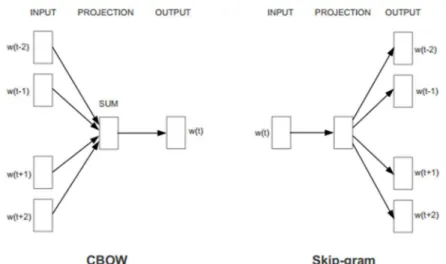
Figure 2.12 shows the architecture of two neural language models proposed by the

authors.

The Continuous Bag-of-Words (CBOW) neural language model predicts the current

word based on the context, and the Skip-gram model predicts the neighborhood words given

the current word.

The similarity between the words whose distributed representations are generated by

these models can be measured using a word-offset technique where simple algebraic

operations are performed on the word vectors. It was shown for example that the vector

(”King”) minus vector (”Man”) plus vector (”Woman”) results in a vector that is closest to

the vector representation of the word “Queen” [Zweig, Mikolov, & tau Yih, 2013].

Figure 2.13 shows a pictorial representation of this example.

In ANN models, the initial values of the network parameters determine the quality of

the learned representations. The same model trained with the same data set using different

Figure 2.13. Algebraic operations on word vectors.

Figure 2.12. Architectures of the CBOW and Skip-gram neural language models.

(48)

initial values for the network parameters can yield different solutions that differ substantially

in quality. Different initial values will bias the learning algorithm to develop some type of

feature detection units at the hidden layers, but not others [Golden, 1996].

In the context of NLP, the use of word embeddings, in the models that consider the

words as the text building blocks, can be viewed as a prior knowledge information strategy

[Gülçehre & Bengio, 2013].

Although some controversies exist about the ability of the word embeddings to capture

semantics of word sequences, there are experiments showing that their use can improve the

(49)

23

Chapter 3

Related Work

In this chapter, we present the related work that apply or develop similar concepts used in

this work. In the course of our research, we made an extensive literature review including

tens of papers, books and online references, but we present only the works that are closer

related to our work. We summarize five works that employ CNN architectures to solve the

text categorization problem.

In Kalchbrenner et al. [2014], the authors proposed a deep CNN architecture to make

semantic modelling of sentences. The model is named Dynamic Convolutional Neural

Network (DCNN). It is based on the architecture of a Time Delay Neural Network (TDNN)

[Collobert & Weston, 2008]. The authors addressed the limitations of TDNN while

preserving its advantages.

The proposed deep CNN architecture has four layers. In the first layer, the input

sentences are represented using word embeddings initialized using a pre-trained

unsupervised model that predicts the contexts of occurrence for the words [Turian, Ratinov,

& Bengio, 2010]. In the second and third layers, the resulting representations from the

previous layers are convolved by a set of filters. The convolution operators are followed by

dynamic k-max pooling and non-linearity operators. The term dynamic means that the

number of the k maximum values selected by the pooling operators changes according to the

sentence size and to the layer level where the operation happens. The output of the third

layer is fully connected to a softmax non-linearity layer that predicts the probability

distribution over the classes given the input sentence.

The network was trained to minimize the cross-entropy of the predicted and true class

labels distributions by backpropagation using mini- batches. The 1D convolution operator

was implemented using a Fast Fourier Transform function. The code was implemented in

(50)

24 CHAPTER 3. RELATED WORK

The authors tested the DCNN in four experiments: small-scale binary and multi-class

sentiment prediction, six-way question classification and Twitter sentiment prediction by

distant supervision. The network achieved excellent performance in the first three tasks and

the error reduction with respect to the strongest baseline was greater than 25% in the last

task.

Although their model deals only with sentences, the architecture proposed by the

authors inspired most of the works that use the CNN architecture in the NLP domain,

including our work. Our model accepts input texts of any size, which makes it usable in real

NLP applications.

In Kim [2014], the author proposed four variants of a CNN architecture based on the

work of Bottou et al. [2011]. The proposed CNN architecture has three layers. The four

architecture variants are created changing the way that the word representations are

initialized and updated during the training.

In the first variant, the word representations are initialized randomly and updated

during the training. In the second variant, the word representations are derived from Google

pre-trained vectors (Word2Vec) and they are not updated during the training. The third

variant is the same as the second one, except by the fact that the word representations are

updated during the training. The fourth variant is the innovation proposed by the author. It

is a mixture from the second and third variants. It creates the concept of channels. Each

channel has its own copy of pre-trained word representations. In one channel, the word

representations are updated during the training, and, in the other channel, they are not

updated.

The author made experiments with seven data sets. Five of them are for sentiment

analysis tasks on user reviews. The performance of the models was compared with strong

base lines like DCNN [Kalchbrenner, Grefenstette, & Blunsom, 2014]. The proposed models

improved upon the state of the art on four out of seven tasks.

The results showed that unsupervised pre-training of word vectors is an important

ingredient in deep learning models for NLP tasks. To avoid overfitting on one specific task,

one can use two channels for the word representations. One is kept static and the other one

is optimized for the specific task that the model is being trained.

Their model also deals only with sentences and, although it has three layers, it is not

(51)

CHAPTER 3. RELATED WORK 25

representations learned by their model is limited because of the lack of depth. Our model

overcomes these limitations using a deep architecture.

In Johnson & Zhang [2015], the authors proposed a shallow CNN architecture using

high dimensional word representations. The convolution operator is applied over sequences

of words called regions. Two variants of high dimensional word representations are used.

One of them is the traditional one-hot vector. The other one, is named bag of words CNN.

In this variant, the words of a region share the same vector representation, where each

position of the vector represents one index of the vocabulary. This approach is a balance in

the trade off between the representations high dimensionality and the order of the words. It

preserves the order of the regions in the sentence but the order of the words in each region

is lost.

The models were implemented using the C++ programming language and they explore

the parallel processing power of the GPUs. Two data sets of user reviews and one of topic

classification are used to compare the performance of the model with other strong baseline

algorithms. The results showed that the proposed architecture achieved an excellent

performance compared with the state of the art algorithms that use low dimensional

pre-trained word representations.

Although the use of an efficient implementation combined with a powerful GPU

makes it feasible the adoption of one-hot representations, the lack of context of this type of

representation makes it harder to their model to extract good semantics from the text. Our

model makes use of the word embeddings as the initial representations for the vocables and

updates them in the training process. This strategy helps our model to extract good semantics

from the text, starting with generic representations and adjusting them to the context of the

specific task.

In Denil et al. [2014], the authors proposed a deep CNN architecture that explicitly

extract representations for the input text at the sentence and document levels. The network

has four layers and it is similar to the one presented in Kalchbrenner et al. [2014], except for

the fact that, in the third layer, the sentence representations are concatenated to form the

document representation. The convolution, k-max pooling and non-linearity operations are

the same used in Kalchbrenner et al. [2014].

The innovation introduced by the authors is the use of a deconvolution technique used

(52)

26 CHAPTER 3. RELATED WORK

activations in convolutional neural networks [Taylor, Fergus, & Zeiler, 2011]. To generate

the saliency map for a given document, the authors applied the same technique used in

Simonyan et al. [2013].

The authors proposed a way to measure the extraction quality of the most relevant

sentences using them as a summarization for the reviews of the IMDB data set. The model

is trained using the whole text of the reviews and the accuracy of the predicted sentiment is

compared with the accuracy of the model trained using only the sentences extracted through

the deconvolution process. The results show that the proposed model outperforms the

baseline methods on the task of extracting the most relevant sentences from text documents.

Although the architecture of their model induces the creation of a hierarchy of

representations, as our model does, the use of only two convolutional layers and the

restriction on the number of words of the input text make the use of their model restricted to

documents of small size. Our model has three convolutional layers and accepts input texts

of any size, which makes it usable in real NLP applications.

In Zhang et al. [2015], the authors proposed a deep CNN architecture for text

categorization using features extracted from character level representations. The network has

nine layers composed of six convolutional and three full-connected layers.

In the input layer, it is created a representation for the input text using the one-hot

encoding of the 70 alphabet symbols that represents the last 1014 text characters. The first

six layers are made up by a sequence of 1D convolution, non-linearity and max pooling

operators. The last three layers are made up by a sequence of linear and dropout operators.

The last layer has a log softmax operator that gives the class labels log probabilities for the

input text representation. The gradients are obtained by backpropagation and the

optimization is done through Stochastic Gradient Descent (SGD) using mini-batches.

To evaluate their model, the authors built eight large-scale data sets. The model was

trained using these data sets to make sentiment analysis and topic classification tasks. The

authors implemented traditional models such as bag of words, n-grams and their TFIDF

variants, and deep learning models such as word-based CNNs and LSTM to be used as

baselines. The character-level CNN models achieved the state of the art performance on four

of the eight tasks.

The use of characters as semantic units demands a huge number of samples to their

(53)

CHAPTER 3. RELATED WORK 27

knowledge principle making use of the word embeddings as the initial representations for

the vocables. This strategy makes our model learn good semantics using significantly less

(54)

28

Chapter 4

Model

In this chapter, we detail the architecture of our model starting by presenting an overview of

the data flow and describing the text encoding mechanism, then we exam the design of the

deep architecture and finally we talk about the network optimization algorithm used to

update the network parameters.

4.1 Data Flow

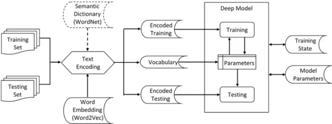
Figure 4.1 presents a flowchart representing the data flow of our model. The data sets are

split in training and testing sets. The vocables occurring in the training set are used to

generate the vocabulary in the text encoding process. The word embeddings are read from a

binary file obtained from a pre-trained model.

(55)

CHAPTER 4. MODEL 29

We implemented two models. The WordNet semantic dictionary corpus is used in the

Deep NLP WordNet model to get synonyms for the vocables in the text encoding process.

The doted lines in the chart denote that the WordNet corpus is not used in the Deep NLP

model.

The vocabulary generated by the text encoding process is used to encode the texts of

the training and testing data sets and it is stored in a binary file that will be loaded by the

deep CNN. The encoded texts of the training and testing data sets are also stored in binary

files that will be used by the deep CNN in the training and testing process. The updating of

the vocabulary representations can be enabled in the training process.

The training state and the network parameters are saved in binary files, so they can be

loaded later in the testing process.

4.2 Text Encoding

The first step in the text encoding process is the text tokenization. Because of our model

explicitly creates intermediate representations for sentences, we first tokenize the text into

sentences, then we tokenize the sentences into words.

The second step in the text encoding process is the vocabulary generation. There are

two steps in the process of building the vocabulary. The first step is to select the vocables

that will compose the vocabulary. In compliance with the principle that the content of the

testing samples should not be viewed by the model before the testing phase, we take into

account only the vocables present in the training samples to build the vocabulary. In this

step, there is an important decision to be made, the vocabulary size.

Because our model learns its parameters in a supervised way and the vocable initial

representations are considered parameters of the network, the vocabulary size has a huge

impact on the number of parameters that have to be learned by the model.

Although there is not a rule of thumb to determine the vocabulary size, one point that

must be considered is the equilibrium between the number of training samples per class and

the number of parameters that have to be learned. To constraint the vocabulary size, we use

the strategy of selecting only the vocables that appear in the training samples at a minimum

(56)

30 CHAPTER 4. MODEL

The second step in the vocabulary generation process is to assign an initial

representation to the vocables. In our model, the vocable initial representations are obtained

from a pre-trained unsupervised neural language model publicly available2 (Word2Vec).

These initial representations are adjusted to the specific context of the training samples

during the training phase.

When a vocable is not found in the Word2Vec, we assign a random value to its initial

representation. In the model implemented using the WordNet corpus, before assigning a

random value to the initial representation of a vocable, we first try to find a WordNet

synonym, lemma or stem whose vocable is present in the Word2Vec.

The WordNet is a large lexical database of English. Nouns, verbs, adjectives and

adverbs are grouped into sets of cognitive synonyms (synsets), each expressing a distinct

concept. Synsets are interlinked by means of conceptual-semantic and lexical relations. The

WordNet’s structure makes it a useful tool for computational linguistics and natural language

processing [Miller, 1995].

The last step in the text encoding process is to associate each text word of the training

and testing samples with its correspondent vocable in the vocabulary. This association is

made assigning to each text word an integer value that is the index of its correspondent

vocable present in the vocabulary.

Instead of ignoring the words whose vocables are not present in the vocabulary, we

assign to them the index of one of the generic vocables specifically created for this purpose

(#NUMBER#, #SYMBOL#, #UNKNOWN#). In the model implemented using the

WordNet corpus, before assigning the index of a generic vocable to a unknown word, we

first try to find a WordNet synonym, lemma or stem whose vocable is present in the

vocabulary.

This strategy enhances the robustness of our model through the generalization of its

learned representations. Even when the model encounter a text with many vocables that it

cannot find in its vocabulary, it is able to replace them by some cognitive synonym that is

present in the vocabulary. This is similar to what the humans do when they encounter an

unknown word in a text. They search the unknown word in a dictionary or thesaurus and

(57)

CHAPTER 4. MODEL 31

replace it by a word whose semantic is already known in a similar context [Gülçehre &

Bengio, 2013].

4.3 Deep Architecture

The design of the network architecture of our model is inspired by the deep CNN

architectures used in the computer vision domain [LeCun, Bottou, Bengio, & Haffner, 1998]

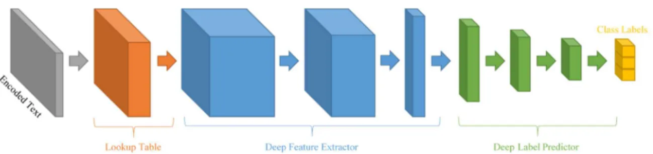
[Krizhevsky, Sutskever, & Hinton, 2012]. Figure 4.2 shows a diagram with the main

components of our model architecture.

Our model implements a sequential standard feedforward architecture. The model is

made up by seven layers that can be grouped into three main components. The first

component is the lookup table. It stores the vocable representations assigned by the

vocabulary building process. This component is responsible for translating the word

encodings into word embeddings. The vocable initial representations are obtained from the

publicly available3 pre-trained Word2Vec binary file using 300-dimensional vectors.

Because these representations are updated in the training phase, this component has the

larger number of the network parameters.

The second component of our model architecture is the deep feature extractor. This

component is responsible for extracting complex features from the text. Because we adopted

the sentence compositional approach, we force the text to pass through layers that explicitly

create intermediate representations for the sentences. At the upper layers of this component,

the sentence representations are concatenated to create the text representation. This

3_{https://code.google.com/archive/p/word2vec/}

A robust deep convolutional neural network model for text categorization

Universidade Federal de Minas Gerais

Instituto de Ciências Exatas

Programa de Pós-Graduação em Ciência da Computação

A ROBUST DEEP CONVOLUTIONAL NEURAL

NETWORK MODEL FOR TEXT CATEGORIZATION

Edgard de Freitas Júnior

VOLUME I

A ROBUST DEEP CONVOLUTIONAL NEURAL

EDGARD DE FREITAS JÚNIOR

A ROBUST DEEP CONVOLUTIONAL NEURAL

NETWORK MODEL FOR TEXT CATEGORIZATION

A

:

A

A

V

Belo Horizonte

Acknowledgments

Resumo

Abstract

List of Figures

List of Tables

List of Acronyms

Contents

Chapter 1

Introduction

1.1

Deep Learning Models

1.2

Convolutional Neural Network Models

1.3

Data Representation

1.4

Compositionality

1.5

Depth

1.6

Objectives of this Work

1.7

Contributions of this Work

1.8

Organization

Chapter 2

Background

2.1

Neural Networks

2.2

Neocortex Deep Structure

2.3

Deep Learning

2.3.1

Depth Matters

2.3.2

The Renascence

2.3.3

CNN Architecture

2.4

Word Embedding

Chapter 3

Related Work

Chapter 4

Model

4.1

Data Flow

4.2

Text Encoding

4.3

Deep Architecture