MAPPING FOREST STAND COMPLEXITY FOR WOODLAND CARIBOU HABITAT
ASSESSMENT USING MULTISPECTRAL AIRBORNE IMAGERY
W. Zhang a, *, B. Hu a, M. Woods b a
Department of Earth and Space Science and Engineering, York University, 4700 Keele St., Toronto, ON, Canada, M3J 1P3 - (wwzhang, baoxin)@yorku.ca
b
Forested Landscape, Ontario Ministry of Natural Resources, 3301 Trout Lake Road, North Bay, ON P1A 3J7 - murray.woods@ontario.ca
Technical Commission II
KEY WORDS: Stand complexity, wildlife habitat, vertical structure, texture analysis, VHR imagery
ABSTRACT:
The decline of the woodland caribou population is a result of their habitat loss. To conserve the habitat of the woodland caribou and protect it from extinction, it is critical to accurately characterize and monitor its habitat. Conventionally, products derived from low to medium spatial resolution remote sensing data, such as land cover classification and vegetation indices are used for wildlife habitat assessment. These products fail to provide information on the structure complexities of forest canopies which reflect important characteristics of caribou’s habitats. Recent studies have employed the LiDAR system (Light Detection And Ranging) to directly retrieve the three dimensional forest attributes. Although promising results have been achieved, the acquisition cost of LiDAR data is very high. In this study, utilizing the very high spatial resolution imagery in characterizing the structural development the of forest canopies was exploited. A stand based image texture analysis was performed to predict forest succession stages. The results were demonstrated to be consistent with those derived from LiDAR data.
* Corresponding author.
1. INTRODUCTION
Woodland caribou (Ranifer Tarandus Caribou) is an important wildlife species ecologically and culturally in Canada. This amazing creature is now at risk and listed as a threatened species provincially and nationally (Ontario Woodland Caribou Recovery Team, 2008). The decline in woodland caribou populations is primarily the result of habitat loss and forest fragmentation which is caused by human interference including spread of agriculture, oil and gas exploration, and mining (McLoughlin, 2003).To protect them from the threat of extinction, it is critical to conserve its habitat conservation. To map the wildlife habitat, the basic idea is to establish a link between the organism’s characteristics and behaviors to the physical habitat (Guisan and Zimmermann 2000). Conventionally, the observation was conducted by field work which has the promising accuracy and generally been used on the local scale. For the past decades, remote sensing techniques played a key role in wildlife habitats mapping, when large spatial information becomes more favourable for broader area analysis while conventional field work is time and labour intensity. (Kerr and Dostoevsky, 2003). The forest inventory map and land use map which generated from lower resolution satellite imagery has been employed as the major data source to map the woodland caribou habitat (Hansen, 2001). In addition to land cover/use maps, other remote sensing products, such as NDVI (Normalized Difference Vegetation Index) images calculated from satellite data with medium to low spatial resolution have been used in other wildlife habitat mapping. However, the map was not usually up to date, and classes from products usually generated for other or generic applications are not best suited for woodland caribou habitat mapping. These
products are not sufficient in characterizing caribou or other wildlife habitat at local (fine spatial resolution) scales and in characterizing sub-canopy vegetation structure relevant to wildlife (Brown, 2006)
Forest vertical structure influences animal–habitat associations and biodiversity significantly (Brokaw and Lent 1999). Recently, studies have focused on the exploitation of aerial digital imagery and high spatial resolution satellite imagery in characterization of forest structure. Song and Woodcock (2002) characterized the sizes of tree crown using the sill of a variogram. Pasher and King (2010) used multivariate texture analysis to produce a continuous map of the structural complexity, which was based on the empirical relationship between the texture variables and field measurements. Kayitakire et. al (2006) used 1-m resolution IKONOS-2 imagery to estimate the forest variables from the texture analysis of Grey Level Co-occurrence Matrix (GLCM). Their results showed that the structure characteristics including top height, circumference, stand density and age variables are correlated to texture variables. Ouma et al (2008) employed grey-level co-occurrence matrix (GLCM) and wavelet transform (WT) texture analysis for the differentiation of forest and non-forest vegetation type using QuickBird imagery. Their results showed that with the combination of GLCM-mean texture (micro-textures) WT- derived texture (macrotextures), the differentiation and classification of the overall vegetation types can be improved.
At longer temporal scale, forest succession is more primary than the structure, as the structure only capture the forest at a certain time period while the forest succession describe the forest development dynamics (Shugart, 2000). In addition, accurate
classifications of forest succession stage at large spatial extents are critical to characterize wildlife habitat (Helle and Monkkonen, 1990). Current Studies have shown that a combined set of LiDAR derived height metrics which characterizing the three-dimensional structure of forest canopies is able to map forest successional stage with a high accuracy (Falkowski, 2009; van Ewijk, 2011).
Although LiDAR data have the ability to reveal the succession stage of the forest stands, the data acquisition and processing take greater cost (Jensen 2005). High resolution remote sensing imagery comes at a greater availability, but no study has explored the relationship in between the image texture and forest succession stages. The objective of this study is to classify forest succession stage through very high resolution multispectral aerial imagery. Specifically, image texture variables which were derived from Gray Level Co-occurrence Matrix and shadow fraction were employed to classify the forest succession stages. In addition, to determine the reliability of the result derived from the image texture analysis, cross validation with LiDAR data was performed. Existed LiDAR metrics was adopted to predict the forest succession stages, and then compared with the classification result generated from imagery for accuracy assessment.
2. STUDY AREA AND DATA SET
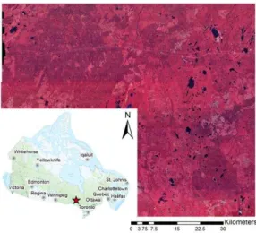
The study area is located near the town of Hearst, Central Ontario, Canada (49.7°N, 83.7°W). Hearst forest falls within the boreal mixed wood region and covers approximately 1.23 million ha; 1.00 million ha of which is productive forest. The study site contains of black spruce (picea mariana), white spruce (picea glauca), balsam fir (abies balsamea), trembling aspen (populus tremuloides) and black poplar (populus balsamifera). The optical imagery which was acquired using a Leica ADS-40 in the summer of 2007 has four spectral bands, blue, green, red and near infrared with a spatial resolution of 0.4 m by 0.4 m. LiDAR data were collected using an Optech ALS50 sensor mounted in a Cessna 310 aircraft in summer 2007 during leaf-on conditions. The LiDAR data were discrete pulse, with an average 1.677 pulses per square meter. Location of the study area is shown in Figure 1 below with a snapshot of the multispectral imagery.
Figure 1. Research area of Hearst Forest, Ontario, Canada
3. METHODOLOGY
To differentiate the stages in forest development, a suite of variables were extracted from the imagery representing the variance within-crown, within-shadow, and canopy level spectral and spatial properties. According to the literature, two approaches have been popular to use, which are semivariograms analysis and Gray Level Co-occurrence Measure (GLCM). Semivariogram contain measurements that relates to forest structure (Lévesque and King, 2003; Treitz and Howarth, 2000). The range of the semivariogram is an indicator of the distance of spatial dependence, often related to the size or scale of dominant objects in the imagery (Curran, 1988; Johansen et al., 2007), and the sill was proved to be an indicator of the total structurally dependent variance in the data that was expected to respond in a manner similar to the texture measures (Johansen et al., 2007). However, semivariogram calculation is complex and computation extensive, which is not suitable for large area mapping. Therefore, the semivariograms for imagery over the whole study area for forest succession stages were not calculated. GLCM approach is adopted for this study. The GLCM variables were calculated first, and used for classifying different forest developing stages.
Shadow fraction, which indicates the tree canopy closure and tree densities, is also an important variable to measure the forest structure. Therefore, shadow fraction was calculated and introduced as an additional variable to the forest development stages classification to test the accuracy improvements. Details of variables extraction and analysis are given in the following paragraphs.
In this study, four general stage of the forest development was adopted. The stand initiation stage indicates where new vegetation becomes established and fully occupies the disturbed site. The young multi-storey stage follows and is mainly characterized by competition among the dominant trees. After the time goes by, young trees start to regenerate and the stand enters the understory re-initiation stage. In the last stage, state as the old growth stage, autogenic and gap-replacing processes create patches large enough for stand initiation to begin (Oliver and Larson, 1996).
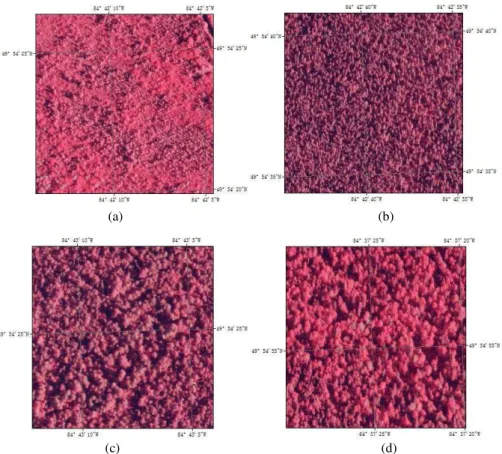
From the entire study area, 20 test areas representing four different succession stages, with the size of 501 x 501 pixels (200m x200m) were subset based on visual interpretation. Example of each forest succession stages are listed in Figure 2. In this study, a size of 400 square meters is used to represent a stand. To capture the spectral and spatial variation within a stand, all 20 test areas are arbitrarily cut into numbers of blocks with a size of 50 pixels by 50 pixels and processed for the image texture analysis.
3.1 GLCM Calculations
For very high resolution aerial imagery, the gaps and shadings in between tree crowns are visible and shown as the spatial variability in image brightness. As the forest developed from young to mature, the amount of the gap and shadings changed as well. Therefore, texture measurements were performed through statistical calculated GLCM.
(a) (b)
(c) (d)
Figure 2: Description of the four forest stand development stages. From top to down and left to right: (a) stand reinitiation, (b)stem exclusion, (c) understory re-initiation, and (d) old growth stage. The false colour composite of the optical imagery covering the study area with the near-infrared band displayed as red, red as green and green as blue
Since the spectral information was not employed in this study, principle component analysis (PCA) was performed to capture the most important information from the image. First component calculated from a PCA of four spectral bands was used for texture measurements. Haralick et al. (1973) first defined 14 texture features that were derived from the GLCM, and eight of them are commonly used GLCM texture measures for remote sensing imagery analysis (Mean, Variance, Contrast, Entropy, ASM, Homogeneity, Dissimilarity, and Correlation). As reviewed from the literature, homogeneity was more effective than the first-order variance in discriminating age classes of Douglas-fir forest stands from IKONOS panchromatic data (Franklin et al., 2001), others also found that the contrast , ASM, entropy and homogeneity measures should be used for forest attributes. (Pesaresi 2000, Cosmopoulos and King, 2004, Kayitakire et al., 2006).
Three parameters controlling the statistics calculated from GLCM were considered in this study, moving window size, displacement and the direction angle. Various values of these parameters have been considered to cover the possible range, while maintaining a manageable number of texture cases. The four main directions (0°, 45°, 90° and 135°) and window sizes 5pixels ×5 pixels, which was intend to capture the variation within crowns. The displacement values were set to 1. The eight texture measures were computed and then further averaged over a plot of 400 square meters, which is considered as the stand size in this study.
Mean
Variance
Contrast
Entropy
Angular Second Moment
Homogeneity
Dissimilarity
Correlation
Where is the th entry of the normalized GLCM matrix; , , and are the mean the standard deviation respectively.
To investigate differentiating all four forest succession stage from the image texture variables, random forest classification was employed. The random forest classifier consists of a combination of tree classifiers where each classifier is generated using a random vector sampled independently from the input vector, and each tree casts a unit vote for the most popular class to classify an input vector (Breiman 2001). Recent applications have shown that random forest is good for classifying hyper spectral remote sensing data, and multisource geographic data (Ham et., al., 2005, Gislason et al., 2006, Lawrence et. al., 2006).
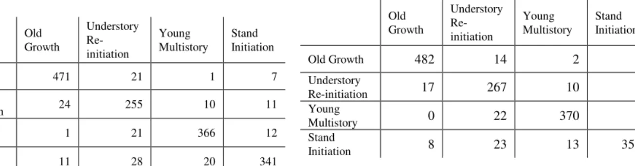
Eight texture variables, Mean, Variance, Contrast, Entropy, ASM, Homogeneity, Dissimilarity, and Correlation, at four direction angles are used together as the 32 parameters in random forest. After the classification, 1433 out of 1600 samples are correctly classified, which is in a result of 89.56 % accuracy. The confusion matrix of the classification result is shown in Table 1.
Old Growth
Understory Re-initiation
Young Multistory
Stand Initiation
Old Growth 471 21 1 7
Understory
Re-initiation 24 255 10 11
Young
Multistory 1 21 366 12
Stand
Initiation 11 28 20 341
Table 1. Confusion Matrix from random forest classification
3.2 Shadow fractions
Different from the low resolution satellite imagery, shadows can be observed in high resolution aerial imagery. The amount of the shadow varied when the tree height, presence of understory and size of the overstory are different. The shadow fraction can be used as one descriptor to measure the structure difference of the forest. In our study, shadow fraction was calculated as the ratio of shaded area to total area within the window size 50 x 50 pixels (20m x 20m). It was derived using the NIR band because it contained the highest contrast between shaded and non-shaded forest areas among all four spectral bands.
Based on the distribution of the histogram, a threshold value was defined to separate the pixels into shades and non-shades groups. The ration between the number of shaded pixel and the total number of pixels within the window is the shadow fraction. Averaged results are shown in Table 2.
As shown in the table 2, each stage of the forest shows different percentage of shadow presences, while the difference in between forest stages is not significant to separate from one another. To test the importance of this texture variable, the shadow fraction was introduced as an additional variable into the classification. Together with the variables derived from the GLCM, the random forest classification accuracy was improved to 92.18%. Also, among all the variables, the shadow fraction
was ranked the third important variable in random forest classification. Overall, the shadow fraction does increase the classification. Specifically, adding the shadow fraction improved differentiate the old growth stage and understory reinitiation, and the stand initiation and young multi-storey. However, it does not improve classify the young multistory and understory re-initation. The confusion matrix of the classification result is shown in Table 3.
Shadow
Fraction St. Dev.
Stand Initiation 0.002287 0.004092
Young Multistory 0.091434 0.038452
Understory Re-initiation 0.051546 0.029982
Old Growth 0.018801 0.015353
Table 2. Shadow fraction derived from NIR band from four forest succession stage
Old Growth
Understory Re-initiation
Young Multistory
Stand Initiation
Old Growth 482 14 2 2
Understory
Re-initiation 17 267 10 6
Young
Multistory 0 22 370 8
Stand
Initiation 8 23 13 356
Table 3. Confusion Matrix from random forest classification after shadow fraction
4. RESULT VALIDATION
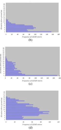
To validate the result from the image texture measurements, a cross validation was applied against the LiDAR data. Since LiDAR data measure the three-dimensional forest structures, such ability makes it possible to classify the forest succession stages. Figure 3 shows the extracted LiDAR points and height distribution.
(a)
(b)
(c)
(d)
Figure 3: Discrete return LiDAR points with height distribution for four forest succession stages. From top to down and left to right: (a) stand initiation, (b)young multistory, (c) understory re-initiation, and (d) old growth stage.
All returns of discrete LiDAR point were utilized for mapping the forest stage. First, DEM which was provided by OMNR was used to normalize the LiDAR points to the ground. To analyze the forest stage at the stand level, the entire area of 5 km by 5 km was arbitrarily cut into numbers of height bins in size of 20m by 20m, and statistical indices within each height bins was calculated. The indices were selected based on the remote sensing and forest ecology literatures that have been popular in terms of analyze the forest structure and development. Such indices include average height, standard deviation of heights, Skewness and Kurtosis of height, the height percentile and height deciles, as shown in Table 5 below.
H_Min Minmum Height
H_Max Maximum Height
H_Ave Average Height
H_SD Standard Deviation of Heights
H_Med Median Height
H_Cov Coefficient of Variation of Heights
H_Skew Skewness of Heights
H_Kurtosis Kurtosis of Heights
H_P1 - H_P9 10th - 90th Height Percentile
H_D1 - H_D9 1th - 10th Height Decile
Canopy Canopy cover = number of 1st return/ Total returns
Table 3: LiDAR derived indices
Empirical model should be built to characterize the forest succession stage. Due to the lack to filed plot, no sufficient information was available to establish a statistical model of using LiDAR data representing forest stage. The model (Equation (1)) reported in van Ewijk et al (2011) to predict Lorey's height for forest succession stage was adopted. Based on their findings, the Lorey's height which is basically the stand tree height weighted by basal area was found to be a good index to separate the young multistory stage from an understory re-initiation stage.
Predicted Lorey's Height = 17.72 + 6.47 H_Skew +0.94 H_Kurtosis +0.80 H_ P9 - 16.59 H_D6 (1) To validate the forest succession stage derived from the texture measurements, 400 samples are employed for the classification from random forest using the previous defined training data. On the other hand, the LiDAR points from the overlapped area from the samples are used to calculate the predicted Lorey’s height. Averaged result is shown in Table 4 below. The results demonstrate that the classification results and LiDAR derived predicted Lorey’s height agree with each other.
Classified Stages Predicted Lorey’s Height
MIN MAX MEAN STD
Stand Initiation 0.08 1.14 0.2563 0.2045
Young Multistory 3.02 7.4 4.9705 0.8615
Understory
Re-initiation 3.4 10.4 6.8701 1.4822
Old Growth 5.89 12.32 9.1612 1.5271
Table 4. Cross validation from the texture measurement classification result with the LiDAR derived predicted Lorey’s height.
5. CONCLUSION
This study shows that using GLCM texture measurements alone can differentiate stages of forest stands development with achieved classification accuracy over 89%. The reason account for that is, as the forest stands develop, the canopy surface will change from smooth to rough, which makes the variation in between canopies measureable from the textural analysis. Specific correlation is sensitive to capture the dependency, thus able to distinguish the homogenous area and the areas with greater variation. In addition, shadow fraction can measure the amount of tree and also the density of the tree crowns. It can be used roughly describe the forest development, but can not distinguish all four stages clearly. However, employed as an additional variable to the variables derived from GLCM, classification result accuracy can be improved to 92%. As the forest developed from young multistory to understory reinitation, the understories are still too small to reflect the sunlight, thus can be taken into account as shadows. Therefore, adding the shadow fraction cannot improve the classification in between these two stages.
In addition, as the LiDAR data has the ability of viewing the forest stands vertically. It was used to statistically describe the
development of the forest. And to further test the accuracy of the classification from the texture analysis, cross validation was performed from the classification result and the LiDAR derived indices. As the class from young to mature corresponding to the predicted Lorey’s height from low to height, the result derived from texture analysis agreed with the LiDAR derived indices. Therefore, the ability of using texture measurements of the high spatial resolution imagery to derive forest complexity information was demonstrated.
Future work will include analyze how GLCM parameters, inter-pixel displacement and the window size influence the estimates of forest structures. At different stages of the forest, the canopy openness, size of the crow/stands will be different. At the early stage of the forest, the trees are more isolated, while in the mature stage, the trees grow into each other, and the overlaps of the tree crown make multiple crowns clustered as one single object. Thus, one window size can not fit all forest stages. Although in this preliminary analysis, a standard window size provides promising result, further analysis will include segmentation process to extract canopy objects. The texture measurements will be processed within each object rather than predefined windows.
6. ACKNOWLEDGEMENTS
The authors gratefully acknowledge Hearst Forest management Inc. for providing the LiDAR data, and Ontario Ministry of Natural Resources for providing the very high resolution aerial imagery. This research was made possible from financial support of Species at Risk Research Fund from Ontario Ministry of Natural Resources and the Natural Sciences and Engineering Research Council (NSERC).
7. REFERENCES
Borre, J. V., Paelinckx, D. C., Mucher, A., Kooistra, L., Haest, B., Blust, G. D., and Schmidt, A. M., 2011. Integrating remote sensing in Natura 2000 habitat monitoring: prospects on the way forward. Journal for Nature Conservation, 19, 116-125. Breiman, L., 2001. Random forests. Machine learning, 45(1), 5-32.
Brokaw, N. V. L., and Lent, R. A., 1999. Vertical structure. Maintaining Biodiversity in Forest Ecosystems. Cambridge University Press, Cambridge, UK, 373-399.
Brown, G. S., Rettie, W. J., and Mallory F. F., 2006. Application of a variance decomposition method to compare satellite and aerial inventory data: a tool for evaluating wildlife-habitat relationships. Journal of Applied Ecology, 43, 173-184. Coops, N. and Bater, C. W., 2009. Remote sensing opportunities for monitoring indicators of forest Sustainability. FREP report, Government Publications, POBox 9452, Stn Prov Govt, Victoria, BC V8W 9V7, 2009.
Cosmopoulos, P., and King, D. J., 2004. Temporal analysis of forest structural condition at an acid mine site using multispectral digital camera imagery. International Journal of Remote Sensing, 25(12), 2259-2275.
Culvenor, D. S., 2002. TIDA: an algorithm for the delineation of tree crowns in high spatial resolution remotely sensed imagery. Computers and Geosciences, 28(1), 33-44.
Curran, P. J., 1988. The semivariogram in remote sensing: an introduction. Remote Sensing of Environment, 24(3), 493-507. Debinski, D. M., Kindscher K, and Jakubauskas M. E., 1999. A remote sensing and GIS-based model of habitats and biodiversity in the Greater Yellowstone Ecosystem. International Journal of Remote Sensing, 20:3281-3291. Falkowski, M. J., Evans, J. S., Martinuzzi, S., Gessler, P. E., and Hudak, A. T., 2009. Characterizing forest succession with lidar data: An evaluation for the Inland Northwest, USA. Remote Sensing of Environment, 113(5), 946-956.
Franklin, S. E., Wulder, M. A., and Gerylo, G. R. 2001. Texture analysis of IKONOS panchromatic data for Douglas-fir forest age class separability in British Columbia. International Journal of Remote Sensing, 22(13), 2627-2632.
Gislason, P. O., Benediktsson, J. A., and Sveinsson, J. R., 2006. Random forests for land cover classification. Pattern Recognition Letters, 27(4), 294-300.
Guisan, A., and Zimmermann, N. E., 2000. Predictive habitat distribution models in ecology. Ecological modelling, 135(2), 147-186.
Ham, J., Chen, Y., Crawford, M. M., and Ghosh, J. 2005. Investigation of the random forest framework for classification of hyperspectral data. Geoscience and Remote Sensing, IEEE Transactions on, 43(3), 492-501.
Hansen, M. J., Franklin, S. E., Woudsma, C. G., & Peterson, M., 2001. Caribou habitat mapping and fragmentation analysis using Landsat MSS, TM, and GIS data in the North Columbia Mountains, British Columbia, Canada. Remote sensing of environment, 77(1), 50-65.
Haralick, R. M., Shanmugam, K., and Dinstein, I. H. 1973. Textural features for image classification. Systems, Man and Cybernetics, IEEE Transactions on, (6), 610-621.
Helle, P. and Monkkonen, M., 1990. Forest successions and bird communities: Theoretical aspects and practical implications, SPB Acedemic Publishing, The Netherlands, pp. 299–318
Johansen, K., Coops, N. C., Gergel, S. E., and Stange, Y., 2007. Application of high spatial resolution satellite imagery for riparian and forest ecosystem classification. Remote Sensing of Environment, 110(1), 29-44.
Johnson, C. J., Alexander, N. D., Wheate, R. D., and Parker, K. L., 2003. Characterizing woodland caribou habitat in sub-boreal and boreal forests. Forest Ecology and Management, 180, 241– 248.
Kayitakire, F., Hamel, C., and Defourny, P., 2006. Retrieving forest structure variables based on image texture analysis and IKONOS-2 imagery. Remote Sensing of Environment, 102(3), 390-401.
Kerr, J. T., and Ostrovsky, M., 2003. From space to species: ecological applications for remote sensing. Trends in Ecology and Evolution, 18(6), 299-305.
Key, T., Warner, T. A., McGraw, J. B., and Fajvan, M. A., 2001. A comparison of multispectral and multitemporal information in high spatial resolution imagery for classification of individual tree species in a temperate hardwood forest. Remote Sensing of Environment, 75(1), 100-112.
Lawrence, R. L., Wood, S. D., and Sheley, R. L., 2006. Mapping invasive plants using hyperspectral imagery and Breiman Cutler classifications (RandomForest). Remote Sensing of Environment, 100(3), 356-362.
Levesque, J., and King, D. J., 1999. Airborne digital camera image semivariance for evaluation of forest structural damage at an acid mine site. Remote Sensing of Environment, 68(2), 112-124.
McDermid, G. J., Franklin, S. E., and LeDrew E. F., 2005. Remote sensing for large-area habitat mapping, Progress in Physical Geography, 29, 4, 449-474.
McDermid, G. J., Hall, R. J., Sanchez-Azofeifa, G. A., Franklin, S. E., Stenhouse, G. B., Kobliuk, T., and LeDrew E. F., 2009. Remote sensing and forest inventory for wildlife habitat assessment. Forest Ecology and Management, 257, 2262-2269. McLoughlin, P. D., Dzus, E., Wynes, B. O. B., and Boutin, S., 2003. Declines in populations of woodland caribou. The Journal of wildlife management, 755-761.
Muinonen, E., Maltamo, M., Hyppänen, H., and Vainikainen, V., 2001. Forest stand characteristics estimation using a most similar neighbor approach and image spatial structure information. Remote Sensing of Environment, 78(3), 223-228. Oliver, C.D., and B.C. Larson, 1996. Forest Stand Dynamics, McGraw-Hill, Inc., New York, 467 p.
Ontario Woodland Caribou Recovery Team. 2008. Woodland Caribou (Rangifer tarandus caribou) (Forest-dwelling, Boreal Population) in Ontario. Prepared for the Ontario Ministry of Natural Resources, Peterborough, Ontario, 93 pp.
Ouma, Y. O., Tetuko, J., and Tateishi, R., 2008. Analysis of co ‐occurrence and discrete wavelet transform textures for differentiation of forest and non‐forest vegetation in very‐ high ‐resolution optical‐ sensor imagery. International Journal of Remote Sensing, 29(12), 3417-3456.
Pasher, J., & King, D. J., 2010. Multivariate forest structure modelling and mapping using high resolution airborne imagery and topographic information. Remote Sensing of Environment, 114(8), 1718-1732.
Pesaresi, M., 2000. Texture analysis for urban pattern recognition using fine-resolution panchromatic satellite imagery. Geographical and Environmental Modelling, 4(1), 43-63. Rettie, W. J. and Messier, F., 2000. Hierarchical habitat selection by woodland caribou: its relationship to limiting factors. Ecography, 23, 466-478.
Serrouya, R. , McLellan, B. N., and Flaac, J. P., 2007. Scale-dependent microhabitat selection by threatened mountain caribou (Rangifer tarandus caribou) in cedar–hemlock forests during winter. Canadian Journal of Forest Research, 37(6), 1082-1092.
Shugart, H.H., 2000. The importance of structure in the longer-term dynamics of ecosystems. Journal of Geophysical Research — Atmospheres, 105, pp. 20065–20075
Song, C., and Woodcock, C. E., 2002. The spatial manifestation of forest succession in optical imagery: the potential of multiresolution imagery. Remote Sensing of Environment, 82(2), 271-284.
Sticker, C. M. and Southworth J., 2008. Application of multi-scale spatial and spectral analysis for predicting primate occurrence and habitat associations in Kibale National Park, Uganda. Remote Sensing Environment, 112, 2170-2186. Treitz, P., & Howarth, P., 2000. High spatial resolution remote sensing data for forest ecosystem classification: an examination of spatial scale. Remote sensing of Environment, 72(3), 268-289. van Ewijk, K. Y., Tritz, P. M., and Scott, N. A., 2011, Characterizing forest succession in Central Ontario using LiDAR-derived indices. Photogrammetric Engineering and Remote Sensing, 77 (3), 261-269