MONITORING AIRCRAFT MOTION AT AIRPORTS BY LIDAR

(1)

MONITORING AIRCRAFT MOTION AT AIRPORTS BY LIDAR

C. Totha,_{*, G. Jozkow}a,b_{, Z. Koppanyi}a,c_{, S, Young}a_{, D. Grejner-Brzezinska}a

a_{Department of Civil, Environmental and Geodetic Engineering, The Ohio State University, 470 Hitchcock Hall, 2070 Neil Ave.,} Columbus, OH 43210, USA - (toth.2, jozkow.1, koppanyi.1, young.1460, grejner-brzezinska.1)@osu.edu

b_{Institute of Geodesy and Geoinformatics, Wroclaw University of Environmental and Life Sciences, Grunwaldzka 53, 50-357} Wroclaw, Poland - grzegorz.jozkow@igig.up.wroc.pl

c Department of Photogrammetry and Geoinformatics, Budapest University of Technology and Economics, 3 Műegyetem rkp., Budapest, H-1111, Hungary - zoltan.koppanyi@gmail.com

Commission I, ICWG I/Va

KEY WORDS: LiDAR, object detection, pose estimation, motion estimation, airport safety

ABSTRACT:

Improving sensor performance, combined with better affordability, provides better object space observability, resulting in new applications. Remote sensing systems are primarily concerned with acquiring data of the static components of our environment, such as the topographic surface of the earth, transportation infrastructure, city models, etc. Observing the dynamic component of the object space is still rather rare in the geospatial application field; vehicle extraction and traffic flow monitoring are a few examples of using remote sensing to detect and model moving objects. Deploying a network of inexpensive LiDAR sensors along taxiways and runways can provide both geometrically and temporally rich geospatial data that aircraft body can be extracted from the point cloud, and then, based on consecutive point clouds motion parameters can be estimated. Acquiring accurate aircraft trajectory data is essential to improve aviation safety at airports. This paper reports about the initial experiences obtained by using a network of four Velodyne VLP-16 sensors to acquire data along a runway segment.

1. INTRODUCTION

Safety in air and land are equally important in commercial aviation. A less known fact is that a large number of accidents, including fatalities, happen at airports where aircrafts collide with each other on the ground. In particular, this is the case with older airports which were designed for smaller aircraft and less traffic. Obtaining reliable and accurate navigation information from landing and taxiing aircraft is difficult. Airport authorities use radar to monitor airplane traffic, which provides only coarse positioning and almost no attitude information; clearly, adequate for traffic control. In contrast, aircrafts, equipped with sophisticated navigation systems based on GPS and IMU sensors, have accurate position and attitude data onboard, but they do not share them with airport management and aviation authorities. Consequently, independent sensing systems, requiring no cooperation from the aircraft is needed to acquire information in volume.

Accurate aircraft trajectory data for all aircraft motion at an airport could provide essential information for many purposes. First, it can be used to analyze the driving patterns of pilots under various conditions, and thus better understand the risk of aircraft motion on runways and taxiways, such as centerline deviation, wingspan separation, etc. Second, modeling aircraft trajectory can improve airport and even aircraft design. Finally, this information can be used to assess airport safety readiness, develop better airport standards, and support pilot education and training (Hall Jr et al., 2011).

Remote sensing technologies offer a simple, yet reliable way to acquire information of aircraft motion at airports. Sensors can be deployed around runways and taxiways, and precise trajectories

* Corresponding author

can be obtained without any assistance from the aircraft. To study taxiing behavior, Chou et al. (2006) used positioning gauges to obtain data at the Chiang-Kai-Shek International Airport, Taiwan. The gauges recorded the passing aircraft’s nose gear on the taxiway. Another study by FAA/Boeing investigated the 747s’ centerline deviations at JFK and ANC airports (Scholz, 2003a and 2003b). They used laser diodes at two locations to measure the location of the nose and main gears. Another report deals with wingspan collision using the same sensors (Scholz, 2005). The sensors applied and investigated by these studies allow only point type data acquisition; detecting the light bar passing.

Imaging sensors are especially effective to acquire large volume of data to extract objects, such as aircraft bodies, and then track them based on image sequences. In particular, LiDAR (Light Detection and Ranging) is a suitable remote sensing technology for this type of data acquisition, as it directly captures 3D data and is reasonably fast. For any scanning system, where the data is continuously acquired, motion artefact happens to any object where there is any relative motion between the sensor and the object. Consequently, the image of the moving object is distorted due to motion. If the object size/shape is known, this phenomenon can be beneficial to estimate motion parameters, such as velocity. In this study, the feasibility of using four profile laser scanners is investigated for aircraft body motion estimation, primarily focusing on heading and velocity estimation.

This study is a continuation of our previous work. In Koppanyi and Toth (2015), the feature extraction and parameter estimation methods are introduced, here experiences using a multisensory configuration are reported.

(2)

2. LIDAR SENSOR NETWORK

2.1 Hardware components of the single sensor unit

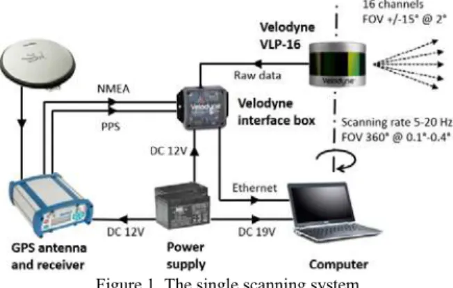
The core data acquisition system is built around the Velodyne VLP-16 profile laser scanner. Since the time information is critical for any data fusion, such as estimating the velocity from the point cloud, the scanner receives navigation messages (NMEA) and the 1PPS (Pulse Per Second) timing signal from a GPS receiver via the scanner interface box. The GPS time stamp provides highly-accurate absolute time, and thus, the system can be further extended, for example, by adding other sensors. The data containing the scanning observation and time information are recorded by a computer. The scheme of the single scanning system is shown in Figure 1.

Figure 1. The single scanning system

For the testing purposes, the system was built in a portable prototype version to check its performance with no consideration given for an optimized implementation. For that reason, it is self-contained; it has its own power supply, the data is stored locally during the scanning period, etc.

2.2 Location and orientation of the scanning units

The most important question that needs to be answered is the optimal location and orientation of the scanner with respect to the runway or taxiway; the acquired data should be sufficiently rich in information to extract the movement parameters of aircrafts of different sizes and moving with different velocities. In simple terms, the more points obtained from an aircraft, the more reliable the parameter estimation.

There are two basic orientations for the Velodyne VLP-16 sensor either vertically or horizontally oriented rotation axis. In the case of vertical orientation, the scanner should be located very close to the runway edge to allow for obtaining useful data from most of the multiple laser diodes. In this orientation, points are acquired in horizontal scanning profiles along the aircraft body, and the separation of the profiles on the aircraft body depends on the distance between the sensor and the aircraft. For example, scanning an aircraft from a distance of 30 m, the sensor laser diode separation of 2°, results in a vertical separation of profiles on the aircraft body of about 1 m, in which case only a few scanning profiles can be obtained for a small aircraft. For that reason, the scanner in such orientation must be placed as close to the runway as possible. For a vertically oriented scanner with a tilt of 15°, Figure 2 shows the observation height range and the number of profiles for a small aircraft at three distances from the scanner. The benefit of the vertical orientation is the large field of view (FOV), allowing scanning a large part of the object space

along the runway direction; note the sensor has a ranging limitation.

Figure 2. Height observation range and profiles for a small aircraft with a vertically oriented Velodyne VLP-16 (15° tilt)

Investigation by Koppanyi and Toth (2015) using a Velodyne HDL-32E sensor and by Dierenbach et al. (2015) based on simulated data showed the benefits of horizontally orientated profile scanners. The Velodyne VLP-16 scanning rate of 10 Hz results in 0.2° separation between consecutive shots of a single laser diode, equaling in a linear separation around 0.1 m for a scanning distance of 30 m. Clearly, this orientation allows to acquire larger number of points across the aircraft body than the vertically oriented sensor. The limitation of horizontal rotation, however, is the small horizontal FOV, and, consequently, only a small section of the runway/taxiway can be monitored. The FOV can be slightly improved by changing the azimuth of the scanning rotation axis with respect to the runway, or increasing the distance to the runway. Of course, the latter will also increase the point spacing along both directions. Similarly to the vertical sensor orientation, the sensor’s range limitation makes the monitoring larger area impossible at some point.

In addition to the discussion on the scanner orientation and distance with respect to the runway, the determination of the optimal height of the scanner needs to be mentioned. On one side, the scanner should not be placed directly on the ground, as it prevents the acquisition of data from the runway that may be beneficial in subsequent processing. On the other side, it cannot be placed too high, as it will increase the chance for collisions with aircraft wings. Since airport regulations strictly control the installation of objects around runways/taxiways, the highest legally allowable height should be used for the sensor. The airport signal lights around runways/taxiways are placed on short poles of about 0.5 m length, and thus, similar poles and heights can be used to install the scanners.

2.3 Collocated scanning units

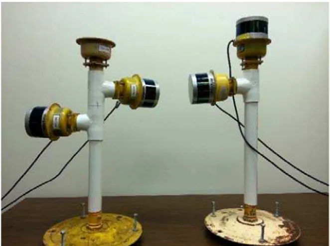
The limitation of a single scanner position and orientation with respect to the runway observability can be mitigated by using multiple scanning units that can monitor different sections of the runway. This multisensory solution is investigated here by building a system from 4 identical Velodyne VLP-16 laser scanners. The LiDAR sensors were arranged in two pairs installed at two locations along a runway. The first pair contained 2 scanners with horizontal orientation, and, to increase the horizontal FOV, the orientation of the rotation axes differed by 30°, see left unit in Figure 3. The second pair, see right unit in ISPRS Annals of the Photogrammetry, Remote Sensing and Spatial Information Sciences, Volume III-1, 2016

(3)

Figure 3, consisted of one horizontally oriented scanner and one with vertical orientation.

Figure 3. Two sets of scanning units

An additional advantage of using two sets was that the number of the prototype hardware components could be lowered, such as the number of GPS receivers and antennas, as the navigation message and timing pulse can be split for sensors, etc. The location of the scanners with respect to the runway, including typical distances is shown in Figure 4. Note that the Velodyne VLP-16 scans 360° around its rotation axis, but the not useful parts of scans (behind scanners) are not shown in Figure 4.

Figure 4. Four scanner configuration (drawing not to scale)

The sensor arrangement shown in Figure 4 was chosen for the initial data acquisition, as it provided sufficient diversity in data from the perspective of the point cloud processing and motion estimation. Obviously, units can be placed at different distances from the runway, at different distances from each other, at different orientation with respect to the runway, or even on the opposite side of the runway, etc. Once the full evaluation of the data has been completed, a new refined sensor configuration may be developed to support further testing. Obviously, for a real permanently deployable system, more scanners and more complex configurations may be considered.

2.4 System calibration

The geometrical calibration of the sensors is essential to obtain point clouds of good internal and absolute accuracy. For that reason, first the internal calibration of each scanner should be performed, and then the relative and absolute orientation of the scanners need to be established.

2.4.1 Velodyne VLP-16 internal calibration: Raw measurements of the Velodyne VLP-16 scanner need to be corrected to achieve the highest accuracy point coordinates with respect to the scanner origin. The calibration model for the Velodyne VLP-16 is identical to the Velodyne HDL-32E or HDL-64E S2 scanners, except the 6 calibration parameters, including range scale factor and offset, horizontal and vertical offsets and angular corrections, are determined for only 16 laser sensors (diodes). All sensors are shipped with factory calibration, but new calibration may be performed by the user to improve internal accuracy of the point cloud. For example, the laboratory calibration method, based on observing planar surfaces from different scanner locations, proposed by (Glennie and Lichti, 2013), can be used.

2.4.2 Orientation and position of the scanners: To transform all points to the same coordinate system, either using a local frame or an absolute mapping frame, the orientation and position need to be known for each scanner in the same frame. The direct determination of the sensor spatial relationship is not possible at high accuracy, and therefore, indirect methods must be used. There are many approaches for point cloud co-registration, however, many of them require a measurable overlap between point clouds that may not be feasible for the developed system here. For example, the lack of objects other than the ground surface of the airfield in the scanning range in the given scanner orientation (see Scanner 1 and Scanner 2 in Figure 4) results in non-overlapping point clouds. For that reason, other methods need to be applied.

The orientation of point clouds was performed in two steps. First, scans are aligned to the surface of the runway and then rotated according to a known azimuth. For the simplicity, in many cases, it can be assumed that the surface of the runway is planar and horizontal, otherwise, additional measurements are necessary to estimate the normal vector of the runway parts observed by each scanner. Then the normal vectors are estimated based on the non-transformed point clouds in the areas corresponding to the runway parts. Based on the pair of corresponding normal vectors, the point cloud can be rotated to match the runway surface, leaving only the azimuth unknown. This problem can be solved by finding and using straight objects in the point cloud. For example, the pavement marks on the runway seem to be a good choice. The paint of the marks is much more reflective than the runway/taxiway surface making these lines clearly visible in the point cloud, see Figure 5. The rotation angle/azimuth can be found by estimating the direction of the runway mark lines in the point cloud and measuring it in the field.

Figure 5. Intensities of taxiway mark lines in the point cloud for horizontally (top) and vertically (bottom) oriented scanners ISPRS Annals of the Photogrammetry, Remote Sensing and Spatial Information Sciences, Volume III-1, 2016

(4)

The above presented absolute orientation determination is a straightforward solution, and was suitable for this investigation; if more accurate orientation is necessary, temporary planar targets/objects around the maximum range and in the FOV of multiple scanners can be added to increase the robustness. The scanner positions can be determined by direct field measurements of the scanner locations in the absolute reference frame, such as by GPS or in a local reference frame, e.g. with respect to the runway. Obviously, the scanner origins are not accessible, yet measurements can be referred to other arbitrary chosen scanner origins and then reduced by offsets estimated by laboratory survey.

3. MOTION ESTIMATION

Pre-processing of point clouds is necessary, as the feature extraction algorithm requires only the points that are reflections from the aircraft. This can be achieved by removing points that are outside of a predefined space; where the scanner cannot see the aircraft. For example, all points with too short range or having certain scanning angle can be easily removed. The classical filtering method based on scanning the object space without any moving and non-moving aircraft in the observation space to obtain an average static scene can be to subsequently extract only the moving objects from the dynamic frames. During the testing phase, the point clouds were filtered outside the cube aligned to the runway and subtracted from static background scene.

The estimation of the aircraft motion parameters includes several processing steps. The general idea is to reconstruct the object geometry using a dynamic model of the motion, which is based on the distorted point cloud due to movement of the aircraft. Assuming a constant velocity and heading of the aircraft body, the point cloud model of the aircraft can be properly reconstructed form the point clouds of different time epochs. The velocity and orientation values are available using the following dynamic model:

∆ ∗ ∆ cos ∗ ∗ ∆

∆ ∗ ∆ sin ∗ ∗ ∆ (1)

where

∆ , ∆ are the 2D displacements of the aircraft body, ∆ is the time difference between two scans,

is the unknown constant heading in the sensor coordinate system,

is the unknown constant velocity of the aircraft, , are the and components of the constant velocity.

At a given set of parameters, from the point clouds, the aircraft body can be reconstructed based on these equations. The orderliness of this point cloud determines the correctness of the reconstruction, and thus the problem to be solved is to find the correct movement parameters that minimizes the disorder. In this case, the reconstructed point cloud will have the maximum consistency. The equivalent to minimizing the disorder is the maximization of the reconstructed point cloud consistency. One of the measures of the disorder is the entropy introduced by Saez and Escolano (2005) and that was used to reconstruct underwater scenario using stereo vision (Saez et al., 2006). This method requires initial values of the unknown parameters that are refined in a quasi-random manner. In the approach used in this investigation, the entropy minimization was changed to the minimization of the number of spatial bins (cubes or voxels) decimating the space. The bin is created only if it contains at least one point of the reconstructed model. Another difference is that the algorithm used here estimates only two movement parameters: velocity along movement direction and heading.

This is generally correct for airplanes moving on the airfield for a short period of a time, as fast turns during taxiing and aircraft movements in the air are excluded. More detailed description of the algorithm used in this study can be found in Koppanyi and Toth (2015).

The proposed algorithm provides robust parameter estimation for airplanes moving on the airfield for a short period of a time. The headings and velocities at various times can be estimated using the algorithm on the merged point clouds obtained by the sensors and separated by time windows. Knowing or assuming curved shapes of the motion trajectory allows to determine the continuous , functions of the parameters using regression. Supposing that this curve is modeled by a polynomial, the design matrix is the Vandermonde matrix of discrete times and the solution of the regression problem is the following in terms of least squares formulations:

(2)

where

, are vectors of the estimated coefficients of the velocity and heading curves, respectively,

is the Vandermone matrix of the times,

, are the vectors of the heading and velocity derived from the proposed algorithm,

is the weight matrix.

The weight matrix considers the point numbers within the time window, because better parameter estimation is expected with larger point clouds.

4. TEST DATA ACQUISITION

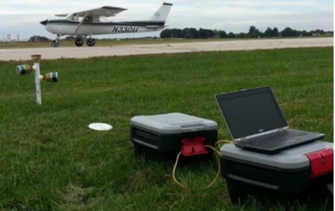
The test data was acquired for a landing Cessna 152 airplane, see Figure 6. Two scanner sets described earlier were placed at the same distance from the runway, separated by 34.8 m, as shown in Figure 4. Such a configuration resulted in observing moving aircraft by maximum of two scanners at any time (one of the horizontal scanners and vertical Scanner 4). At the selected scanning rate of 10 Hz, the time required to observe the moving aircraft by each scanner was about 1.2 s and 7 s for scanners 1-3 and 4, respectively. The point clouds from all scanners were co-registered in the local coordinate system defined by the origin of Scanner 3 and oriented that 0° direction of the Scanner 3 was the Y axis. The local coordinate system orientation and acquired point clouds used in the estimation of movement parameters are shown in Figure 7.

Figure 6. Scanning of a landing Cessna airplane ISPRS Annals of the Photogrammetry, Remote Sensing and Spatial Information Sciences, Volume III-1, 2016

(5)

Figure 7. Acquired point clouds (top view)

Figure 8 shows the point clouds acquired by Scanner 3 for the landing airplane in the period of 1 s; note points obtained by different scanner rotations (frames) have different colors. Looking only at one point cloud (single frame), it is impossible to see the shape of the airplane. However, by adding more frames from all scanners and aligning them perpendicular to the aircraft movement direction, the shape of the airplane can be easily distinguished, see Figure 9.

Figure 8. Point clouds acquired by Scanner 3 (perspective view)

Figure 9. Point clouds acquired by all scanners (rear view)

The visual inspection of the point cloud shown in Figure 9 indicates that for a short period of a time, the Cessna was still in the air, since points acquired by Scanner 1 (red in Figure 9) representing the wings and wheels have larger height than for other scanners. However, this may pose challenges to the processing algorithm depending on the model complexity. On the other hand, the algorithm is not too sensitive to small elevation differences due to the applied relatively large (more than 0.5 m) bin size; note that the maximum elevation from the ground is approximately 0.5 m. For a given bin size, this value is small enough to keep the dynamic model presented by Eq. 1 valid.

5. RESULTS AND DISCUSSION

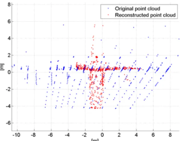
Initially, the velocity and heading were estimated using the method described earlier. Both parameters were calculated every 0.2 s for the 0.5 s and 4 s data acquisition period with a 1 s time window. An example of the reconstructed point cloud (red) with respect to the center of the time window and the originally acquired point cloud (blue) within the applied 1 s time window is shown in Figure 10. Clearly, the shape of the aircraft in the reconstructed model is better visible than in the single frame or in the combined raw point clouds. Note that the model is

incomplete, since scanning was performed only from one side of the runway. In addition, the point cloud density seems to be low for adequately modeling the geometry, yet, for the lower speed of taxiing airplanes, recognition of the aircraft type and model should be possible by measuring characteristic features of the airplane in the reconstructed point cloud.

Figure 10. The captured points (blue) and the reconstructed point cloud (red) within 1s time window

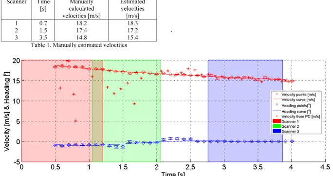
Based on the discrete estimated motion parameters, a 2nd_order and a 4th_{order polynomials were used to model the velocity (red)} and heading (blue) motion curves, respectively, shown in Figure 11. The discrete parameter values from the algorithm with 1 s time window at 0.2 s sampling are depicted by circles with the weighted regression error bars. The red stars show the velocity estimation of a straightforward approach when the velocities are calculated from the consecutive point clouds assuming the aircraft nose is the rightmost point of the clouds. The stripes marked with different colors represent the data availability of the three vertical sensors on the dataset. Note that the horizontal sensor is available during the whole measurement.

The velocity curve in Figure 11 shows a decreasing tendency that is expected during the landing procedure. The velocities from the nose points (red stars) are quite bad in the beginning of the dataset until the second sec epoch that is caused by no backscatters from the nose. The 2nd_{part of these points shows correlation to the} fitted curves that confirms the correctness of the parameter estimation. Heading angles are in the range of about +/– 2° from the runway azimuth. These values are rather realistic considering possible changes of the aircraft attitude during landing.

The estimated velocities are consistent with velocities obtained from manual analysis of the point cloud. The manual evaluation was performed by analyzing the time and position of points reflected from the same, easy to distinguish objects, i.e. airplane wheels in consecutive frames, see Figure 8. The manual velocities were obtained for horizontally oriented scanners separately by averaging velocities from a few frames. The obtained results, shown in Table 1, confirm high consistency with the velocities obtained using the automatic algorithm.

Figure 12 shows the trajectories calculated from the motion curves. The black points on the trajectories mark the data acquisition points. Axes are not equal in terms of aspect ratio to better show the motion in Y direction. The results indicate a swinging pattern with about 20-30 cm maximum deviation from the centerline for the individual trajectories.

(6)

Scanner Time [s]

Manually calculated velocities [m/s]

Estimated velocities [m/s]

1 0.7 18.2 18.3

2 1.5 17.4 17.2

3 3.5 14.8 15.4

Table 1. Manually estimated velocities

.

Figure 11. Velocity (red) and heading (blue) curves estimated from discrete parameter estimations (circles)

Figure 12. Trajectories from the estimated motion curves (not to scale)

6. CONCLUSIONS

Initial results on estimating aircraft motion parameters on runways and taxiways are reported. Data was acquired by four Velodyne VLP-16 scanners, installed along a runway at two locations. One of the sensor pairs had horizontally and vertically oriented sensor axes, providing good FOV in both directions. The other sensor pair had both sensors oriented horizontally with a 30 skew angle to provide larger horizontal FOV. A landing Cessna 152 aircraft was observed multiple times, providing data for the estimation process, which aimed at estimating the aircraft velocity and heading. Results for the velocity estimation used a reference obtained by manual evaluation confirmed a good accuracy. The performance validation of the heading estimate is harder due to the difficulty of acquiring reliable reference data. Nevertheless, the data acquisition method and the developed estimation algorithm have provided encouraging results for a small size airplane with rather slow landing speed.

ACKNOWLEDGEMENTS

Support from the PEGASAS FAA program is greatly appreciated.

REFERENCES

Chou, C., Cheng, H., 2006. Aircraft Taxiing Pattern in Chiang Kai-Shek International Airport. Airfield and Highway Pavement Specialty Conference, April 30 – May 3, 2006, pp. 1030-1040.

Dierenbach, K., Jozkow, G., Koppanyi, Z., Toth, C., 2015. Supporting Feature Extraction Performance Validation by Simulated Point Cloud. ASPRS 2015 Annual Conference, May 4 - 8, 2015, Tampa, Florida, USA.

Glennie, C., Lichti, D.D., 2010. Static calibration and analysis of the Velodyne HDL-64E S2 for high accuracy mobile scanning. Remote Sensing, 2(6), pp. 1610-1624.

(7)

Hall Jr, J. W., Ayres Jr, M., Shirazi, H., Speir, R., Carvalho, R., David, R., Huang, Y.-R., 2011. Risk Assessment Method to Support Modification of Airfield Separation Standards. ACRP Report 51 (prepared under airport cooperative research program,