The role of consumer's risk aversion on price rigidity

,-e

FUNDAÇÃO

GETULIO VARGAS

Ｌｾ＠

FGV

EPGE

,

SEMINARIOS DE PESQUISA

ECONÔMICA DA EPGE

lhe role of consumer' s risk aversion on

price rigidity

SERGIO AFONSO LAGO ALVES

(Banco Central do Brasil)

Data: 16/02/2006

(Quinta-feira)

Horário:

16h

Local:

Praia de Botafogo, 190 - 110 _andar

Auditório nO 1

Coordenação:

The Role of Consumer's llisk Aversion on Price Rigidity*

Sergio A. L. Alves

t

Central Bank of Brazil

Mirta N. S. Bugarin:j:

University of Brasília

Preliminary Version - Comments welcome!

February 7, 2006

Abstract

This paper aims at contributing to the research agenda on the sources of price sticki-ness, showing that the adoption of nominal price rigidity may be an optimal firms' reaction to the consumers' behavior, even if firms have no adjustment costs. With regular broadly accepted assumptions on economic agents behavior, we show that firms' competition can lead to the adoption of sticky prices as an (sub-game perfect) equilibrium strategy. We introduce the concept of a consumption centers model economy in which there are several complete markets. Moreover, we weaken some traditional assumptions used in standard monetary policy models, by assuming that households have imperfect information about the ineflicient time-varying cost shocks faced by the firms, e.g. the ones regarding to inef-ficient equilibrium output leveIs under fiexible prices. Moreover, the timing of events are assumed in such a way that, at every period, consumers have access to the actual prices prevailing in the market only after choosing a particular consumption center. Since such choices under uncertainty may decrease the expected utilities of risk averse consumers, competitive firms adopt some degree of price stickiness in order to minimize the price uncertainty and fi attract more customers fi.'

Keywords: Infiation dynamics, price rigidity, risk aversion, choice under uncertainty, Calvo type model, monetary policy, welfare analysis, DSGE models.

JEL Classification: C73, D43, D81, D82, D84, E31, E52, E58

*The authors are especially grateful to Eduardo Loyo, Il'vIF Executive Director and Professor of Economics (Economics Department of PUC, Rio de Janeiro), for his important suggestions and comments. We also would like to thank Profs Rodrigo Penaloza and Maurício Bugarin, both from the Economics Department of the University of Brasília, and Waldyr Areosa, André Minella, José Álvaro R. Neto and Fábio Araújo, from Central Bank of Brazil, for helpful comments. All remaining errors are our own responsibility. The views expressed here are those of the authors and not necessarily those of the Central Bank of Brazil.

tSenior Advisor at the Special Studies Deputy Governor's Office, Central Bank of Brazil. Phone: (55-61) 3414-3502. E-mail: [email protected]

1

Introduction

This paper aims at contributing to the research agenda on the sources of price stickiness, showing that the adoption of nominal price rigidity may be an optimal fums' reaction to the consumers behavior, even if fums have no adjustment costs. With regular broadly accepted assumptions on economic agents behavior, we show that firms' competition can lead to the adoption of sticky prices as an (sub-game perfect) equilibrium strategy in order to attract more customers. The intuition behind the model formal conclusions are explained as follows.

We introduce the concept of a consumption centers model economy in which there are several complete markets that also compete with each other. Moreover, we weaken some traditional assumptions used in standard monetary policy models, by assuming that households have imperfect information about the inefficient time-varying cost shocks faced by the firms, e.g. the ones regarding to inefficient equilibrium output leveIs under fiexible prices. Moreover, the timing of events are assumed in such a way that, at every period, consumers have access to the actual prices prevailing in the market only after choosing a particular consumption center. Indeed in a real world economy with several consumption centers as supermarkets or shopping malls, for instance, high frequent decisions on which one to choose are made before knowing the actual prices. Since such choices under uncertainty may decrease the expected utilities of risk averse consumers, competitive firms adopt some degree of price stickiness in order to

minimize price uncertainty and 11 attract more customers ". On the other hand, increasing such

a degree reduces the unconditional expected discounted fiow of firms' profit, so there is a trade off between attracting more costumers and reducing profits.

In such a context, we proof two theorems stating that: (a) there is no equilibrium in which households always choose the same consumption center; and (b) the equilibrium degree of price stickiness is the highest, provided that firms have non-negative unconditional expected discounted profit fiows, e.g. the unconditional expected discounted profit fiows will be zero in non-trivial cases. Such a result follows from the two types of competition inputted in the model. The fust one is the traditional monopolistic competition that allows each firm to choose an optimal price that maximizes its expected discounted profit fiow. The second one is the Bertrand fiavor competition played by the consumption centers using the degree of price stickiness in order to be more "attractive" for the households.

1.1

Background literature

Considerable empirical evidence suggests that prices are sticky in the short run. Some pricing behavior studies, carried out among representative firm samples, indicate that several prices

remain fixed on average for more than one quarter1 . This price setting behavior suggests that

prices do not change as frequently as the observed alterations in the state of the economy, which occur more often.

Those facts motivated the development of a broad theoretical research agenda about price stickiness modeling. In order to filter the spectrum of possible theories concerning price sticki-ness, indicating correct ways to be followed by future researches, Blinder et aI. (1998) surveyed

the reasons why firms do not adopt flexible prices among a significative sample of 200 firms in the United States, from several industries. They asked business people about their price-setting practices and their opinions about which academic theories, expressed in laymen's terms,

matched the actual price-setting procedures in United States2 •

It is interesting to note that, although it was never asked whether their costumers were averse to price variation, most of the surveyed firms voluntarily mentioned that changing prices would "antagonize" or "cause difficulties" with their customers, and such a fact would be a strong reason why firms fear to adjust their prices. Indeed, the authors stressed that this issue "carne up so often that figuring out precisely what it means should be a high-priority item on any future research agenda." Surprisingly, Hall et aI. (1997) also stressed that fact that their surveyed firms "stated that physical menu costs of changing prices were a less important source of price rigidity than the need to preserve customer relationships". And at the same direction, Zbaracki et aI. (2004) stated: "Changes in prices harmed the customer perceptions of the firm's reputation, integrity, and reliability."

Nowadays the mainstream in price stickiness macroeconomic modeling, whose main refer-ence relays in Woodford (2003), incorporate adjusting costs, strategic complementarities mea-sures and the presence of differentiated goods, on a monopolistic competition environment. Taking the real business cycle (RBC) analysis structuré, those models focus on the agents optimization problems with intertemporal budget constrains and are so general that the neo-classical or new-Keynesian features are just a result of a particular relationship assumed between the basic preference and technology parameters. Those parameters define the degree of price setting strategic complementarity, among the suppliers of different goods, whose magnitude defines how sticky prices are.

Moreover, the majority of the existing analysis on price stickiness directly assumes a Calvo's

(1983) type source of nominal rigidity or its extensions4 • Brief:l.y speaking, the simplest model

state in ad hoc way that fums maintain unchanged their prices for two consecutive periods

probability a, independently on the other fums' behavior. Such a modelling approach has

been often used in monetary policy analysis for aIlowing a straightforward derivation of the central bank's loss function, as a second order approach of the welfare function, besides a good empirical adherence as well as an easy analytical treatment. As a matter of fact, Calvo's type models may be interpreted as stylized simplifications of the more plausible state dependent

adjustment cost models5 , generating similar results with less analytical effort.

In spite of such appealing features, Calvo's type models have been subjected to some

criti-cism due to the fact that the stochastic process is imposed into the model economy in a rather ad hoc way. Furthermore if firms have no adjustment costs, a Calvo's type economy with time-invariant ineflicient shocks is not eflicient, for under usual assumptions the adoption of flexible prices wiIl be the optimal choice from both the fums and consumers point of view. Therefore, there are no reason why firms would rationaIly submit themselves to a Calvo's lottery. The case of time-varying ineflicient shocks is still inconclusive, depending on whether consumers prefer a f:l.exible price environment or noto

2They confirmed the empirical relevance of the theory in which "firms hold back on price changes, waiting for others to go first", e.g., in which multiple equilibria may arise from the interaction of menu costs and strategic complementarities in price setting. In second place, there were the theory referring to "delaying price increases until cost rise", pointing to some markup procedure on price setting.

3 A good reference on several RBC models can be found in Barro and Sala-I-Martin (1995).

4Good references are Rotemberg and Woodford (1997), Rotemberg and Woodford (1998), Galí and Gertler (1999), Amato e Laubach (2000), Galí et aI. (2001), Clarida et aI. (2002), Woodford (2003), Giannoni e Woodford (2003), Woodford (2004), Galí and Monacelli (2004), Loyo e Vereda (2004), and Alves and Areosa

(2005), among others.

Rotemberg (2002), on the other hand, presented a model in which the probability a of not

adjusting the prices for two periods is determined on an endogenous way. If consumers' utility

functions have a psychological component, regarding the expected degree of firms' altruism, they strongly react to unfair price increases. Hence if consumers have imperfect information about the actual costs, firms will be unwilling to adjust prices so frequently due to the possibility of being interpreted as an unfair pricing setter by the consumers. The key point of this study

is to regard the consumers' behavior as the source of price stickiness, as being suggested by

Blinder et alo (1998). However, his results apply only to unfair price increases, so consumers' aversion to price variations still remains to be carefully understood and analytically treated.

1.2 The paper approach

Within this framework, the present study aims to build a model of pricing behavior in which the degree of the price rigidity is strategically chosen by profit maximizing firms, as an optimal decision to face consumer's risk aversion. Thus, the probability of not adjusting prices is endogenously determined. Moreover, some of the assumptions adopted in the basic Calvo's type model considered in Woodford (2003) are relaxed, allowing for the presence of several (unit

mass) complete markets in the model economy. These markets are herein called consumption

centers. We state that households do not assess the information about the actual state of the economy, in terms of the real firms' costs and prices, prior to each period consumption center choice. Once such a choice is made the actual state of the economy is revealed but consumers

optimal shopping decisions are restricted to the elected consumption center6 . In each of the

following periods, new choices on consumption center are made in similar conditions.

In equilibrium, it will be shown that firms adopt a randomization strategy to decide when to àdjust prices. Such an equilibrium will be found with traditional assumptions about consumers' preferences. As presented further on, price stickiness will be a consequence of the broadly accept assumption of consumers risk aversion, formalizing the research lacuna mentioned by Blinder et

aI. (1998). In such an environment, the price uncertainty of a fiexible price economy decreases

the consumers' expected discounted utility fiow, so competitive firms adopt a price stickiness strategy as a best response in order to attract more clients. On the other hand, increasing price stickiness reduces the present value of firms expected profit fiow. So equilibrium implies that firms increase the price nominal rigidity until the point in which the present value of firms expected profit fiow is zero7 . Consequently, our results represent a plausible solution to the unsolved problem of the case of firms facing time-varying inefficient cost shocks.

This paper is organized as follows. Section 2 presents the necessary modeling extensions

to the Woodford's (2003) basic model, formally deriving the main result of this study, namely the implicitly defined degree of price stickiness in the model economy. Moreover, this section also presents original contributions to the theoretical analysis nominal rigidity sources. Section 3 presents Taylor approximations to the structural results derived in section 2 and introduces some related conclusions. Simulations on the endogenous degree of price stickiness and the volatility of the aggregate variables are also shown in this section. Finally, Section 4 concludes.

2 The Model

In this section, we introduce an extension to Calvo's type basic model. But now competitive

firms strategically choose the degree of price stickiness, which in equilibrium depends on the

economy deep parameters, namely the consumers' risk aversion and the ones related to the production function and the stochastic cost shocks distribution.

Furthermore, it depends on the way monetary policy is conducted. Thus, the Lucas's cri-tique applies in this latter sense. But a similar cricri-tique also comes up. Adapting Woodford (2003) words: since price stickiness depends on the exogenous cost shock distribution, tradi-tional monetary evaluation exercises using macroeconometric models are fl.awed by a failure to recognize that the relations typically estimated, even with quasi-structural equations containing future expectations derived with an ad hoc imposed nominal rigidity source, are reduced-form rather than truly structural relations, for structural changes in the stochastic cost shocks gen-erating process may change the optimal degree of price stickiness chosen by the firms.

As in standard recent literature (see Woodford (2003) for more details), we model a cashless economy, in which there is a monetary unit of account in terms of which prices are quoted. This unit of account is defined in terms of a claim to a certain quantity of a liability of the central bank, which may or may not have any physical existencé.

2.1

Households

In real world, purchasing decisions of great part of goods, as durables, are sufficiently sparse to allow enough time to gather price information before purchases are actually concluded. Thus traditional assumptions stating that consumers know all the prices before consuming is quite a good description of reality. Such an economic decision is exhaustively modeled and its consequences are well understood.

But there are situations in which such a premi se does not work so well. Consumers

fre-quently face the following recurrent questions: which shopping mall should I choose? Or which supermarket? People's habitual behavior is to choose a supermarket before knowing the actual prices, only effectively known when walking through its rows. And doing so, empirical evidence points that after choosing a place to buy, consumers restrict their purchasing decisions only to the goods found in the elected market.

Therefore, the following question arises: how to incorporate such a decision pattern in formal analytical models? And what are the consequent optimal agents decisions?

In an effort to answer such a question, we assume the existence of severa! complete markets, or consumption centers (Cj , henceforth), indexed by j. In each one, monopolist firms i hire

specialized labor force hj,t (i) at nominal wage Wj,t (i) and produce differentiated goods i. As

usual, we assume that i E (0,1) in a unit mass continuum and that individual firm's decisions

have no influence on wages. Each market is then characterized by monopolistic competition. We also assume that firms are subjected to exogenous cost shocks, formalized further on, but none of them are subjected to price adjustment costs.

8 As analytically shown in Woodford (2003), such an approach is justified by two facts:

(a) In an economy in which the central bank uses a short-term nominal interest rate as their instrument, often empirically characterized by central bank reaction functions as Taylor type rules, the old theoretical mo deIs considering money growth targets are not convenient since it is not necessary to first determine the endogenous evolution of money supply in order to understand the consequences, in terms of product, inflation and welfare, of such interest rate rules. Money, prices and interest rates are rather simultaneously determined given a central bank reaction function;

Here, we consider markets transacting non-durable goods, so that the purchase decisions happen with high frequencT. Given the great number of goods and given the decision frequency, it is not reasonable to consider that consumers are informed of ali the prices prior to each period market choices. Not because of information cost, but due to the fact that the period length between consecutive consumption decisions is lower than the necessary to memorize

make optimal decisions based on the huge information setlO •

Therefore, the above consideration leads us to assume that the consumers' buying decision is based on historical data on prices. In other words, we assume that the consumers know the historical average pricing strategy adopted by each firmo In general, this information can be summarized by indexes such as price averages, price volatility and so on.

Even though it seems to be a strong assumption, it captures the observed consumers be-havioral pattern previously exemplified. For illustrative purposes, we can take the traditional

grocery shops as exa,mples of our model's consumption centers. Each itemll _{is sufliciently}

dif-ferentiated and they alI are diversified. Another example would be the set of large shopping malIs, which gather several differentiated firms.

For simplification purposes, we build a model in an environment with only two consumption centers12. Due to such considerations, we make the model's primary assumption:

Assumption 1 In every period, preceding the choice of a consumption center, only historical price patterns are households common knowledge. Hence, they choose a consumption center before they have the information about the prevailing prices of the chosen center. Once this choice is made, their consumption decisions are restricted to the chosen market.

Furthermore, it lis important to make use of some tools from game theory, in particular some concepts and their rationale, for they explicitly handle the agents' rationality. Indeed, the microfounded macroeconomic rational expectations equilibrium concept have their peer in game theory sub-game perfect equilibrium concept, for embedding the same rationale of backward

inductions methodological algorithm: rational expectations optimal decisions in period t are

agents' best responses, given the best responses to be made in the future.

Under certain assumptions, described in Woodford (2003), we may use the concept of a

representative household. In order to characterize its preferences, we define u (.) and v (.)

denoting consumption utility and labor disutility respectively13. It is convenient to make some

regularity assumptions:

Assumption 2 The domains of u (.) and v (.) are strictly positive14 , zn other words u, v

(0,+00) ＭｾＮ＠

9Hence, the model is not proposed to explain the whole economy, but only specific sectors.

lOEven with computer assistance to find which firms are cheaper, time would still be an issue, due to the length of time required by price researches to catalog and release price information.

11 Since the mo dei assumes an infinite number of agents, one may argue that the real world finite number of agents may fiaw the model results. Nevertheless, a known result of Debreu (1975) states that a Walras equilibrium convergence rate to the core, in regular economies, is of order O(1/n). Since Walras equilibria have a finite number of agents in spite of the infinite number of agents of the core, one may conjecture that the problem concerning the number agents may be minimized at least as fast as the actual number of agents.

12 However, the analytical treatment and results can be easily expanded for the case of several consumption centers.

13Note that they are l10t subject to preference shocks, as in traditional literature. AIso, we assume further on the absence of technology shocks in the production function. Such assumptions aim only to simplify the analysis allowing us to better understand the consequences of inefficient time-varying exogenous shocks hitting firms' marginal costs, formally introduced in subsection 2.2. And due to this last disturbance source, the model distinguishes the concepts of natural and steady state products, formally defined in subsection 2.2.l.

.

'

Assumption 3 The function consumption utility u (.) is increasing in consumption, strictly

concave, and its third derivative satisfies Uccc (.)

>

O in its domain. Furthermore, the function labor disutility v (.) is increasing in labor and strictly convex in its domain.

According to Assumption 1, consumption decisions are restricted to the chosen Cj .

There-fore, we may aggregate consumption in such a consumption center considering the Dixit and

Stiglitz (1977) standard way, which assumes a constant elasticity of substitution ()

>

1 among

the differentiated transitioned goods, as shown in equation (1) below, where Cj,t (i) indicates

the consumption of good i from Cj , in period

t .

[

t

9-1

ＱＹｾＱ＠

Cj,t

=

lo

Cj,t (i)-9 di , Vj E {I, 2} (1)

In each period t, after choosing a particular Cj , households gets the instantaneous

consump-tion utility u (Gj,t), e.g. no matter how Cj,t is distributed among each good i from Cj , only the

aggregate consumption in the consumption center is important in terms of preference issues15 .

One can easily derive16 _{the hicksian demand function of good i from C}

j and an expression

for the aggregate price Pj,t in each consumption center, as shown in (2) and (3), below .

. (') _ G. (pj,t (i))-B

c),t 'I, - ),t P

j,t (2)

[

1

1

1:9

Pj,t =

1

Pj,t (i)l-B di (3)

\Vhere Pj,t satisfies Pj,tCj,t =

foI

Pj,t (i) Cj,t (i) di.

In order to capture either deterministic or stochastic (randomizations) choices among each

consumption center, define "/ as the probability of choosing the C1 . This modeling procedure

allows, in turn, to capture deterministic choices by "/

=

O or "/

=

1, as the events in which the

household always chooses C1 or C2 , respectively. Moreover, this probabilistic treatment allows

for possible randomizations, without the need of modifying the corresponding expressions. As a consequence of Assumption 1, the choice of the consumption center can be interpreted as a choice among lotteries, with the corresponding pay off's depending on the prevailing prices

found at the chosen center. Hence, the aggregate consumption Ct from both consumption

centers must satisfy the equality (4), e.g. Ct is the equivalent consumption, under absence of

uncertainty on the lottery choice, which generates the same utility leveI as the one measured

by the expected utility. However, Ct is not a certainty equivalent aggregate consumption, for

it is still a random variable due either to the uncertainty regarding the prices found in each consumption center and to the other random variables present in the model economy.

(4) For simplification sake, we assume as well that the representative household supply labor

only at the chosen consumption center C j . Thus we aggregate the labor force hj,t (i) supplied in

each C_j to produce good i by the same way we did with the aggregate consumption, for there

are similar uncertainties as the previous considered ones. Therefore we aggregate the amount of labor force as indicated below in equation (5).

v (ht (i)) = "/. v (h1,t (i))

+

(1 - ,,/) . v (h2,t (i)) (5)

15Such an assumption is very in line with the one adopted in recent literature.

We may now define

Pt

and Wt (i) denoting the aggregate price and the aggregate wage of

labor force of type i among all consumption centers in period t, respectively, satisfying the

following relations:

(6)

Wt (i) ht (i)

=

'Y 0 Wl,t (i) h1,t (i)

+

(1 - 'Y)

o W2,t (i) h 2,t (i) (7)

As standard, we assume that financiaI assets are evenly shared among all households in

period zero, so complete markets imply in identical budget restrictions for every householdo o.

Moreover, define

Wt

as the nominal financiaI wealth held by the household in the beginning of

period t, Qt,t+1 as the stochastic discounting factor that must exist under absence of arbitrage,

!3

as the preference intertemporal discounting factor, it is the nominal interest rate satisfying

(1

+

it)-l = EtQt,t+1 and IIt (i) as the nominal profit from selling each good i. Also define

Qt;r =

n:=t+l

Qs-l,s.

Regarding the representative household, note that after choosing a Cj in each period t,

the prevailing prices of the chosen center are known. However, expectations regarding future consumption and prices are summarized by CT and Pn for \/T

>

t, for the future choices on

consumption centers are still lottery choices. Hence, the household problem can be formally represented by (8) and its solution depends on the non-ponzi constraint (9).

max

{Cj,t, hj,t(i)} {C7" ,h7"(i)}

s.t. Pj,tCj,t

+

ET [Qt,t+l Wt+l] ::; W t

+

foI (Wj,t (i) hj,t (i)

+

IIt (i)) di

(8)

PTCT

+

ET [QT,T+1 W T+1] ::; W T

+

foI (wT (i) h T (i)

+

IIT (i)) di , \/T> t

(9)

Denote by lj,t and yt aggregate production leveIs to be further discussed. Considering that

all production must be consumed in equilibrium for every period, e.g. Cj,t

=

Yj,t and _{C t}

=

yt,

it is straightforward to solve the problem (8) and obtain the standard shaped Euler equations (10) and (11).

Uc (Yj,t)

P-J, t

Uc (YT )

PT

, \/T

>

t

Note that in period t - 1, the following equation would hold as a consequence of (11).

Uc (yt)

=!3E

[(Q

)-1 Uc (yt+l)]

D t t,t+l n

rt rt+l

(10)

(11)

(12)

Purging equations (10) and (12), we present the new generalized Euler equation (13) asso-ciated to our consumption center economy:

Uc (yt)

=

Uc (Yl,t) = Uc (Y2,t)

=

At

Where

A _t =

f3E

_t

[(Q

_t,t+1 )-1 Uc (Y;+1)]

D

ít+1 (14)

The last results lead us to an interesting interpretation. Even after the choice of a consump-tion center, the expectaconsump-tions about future aggregate consumpconsump-tion and prices do not change and are the same as the ones prevailing just before that choice. Furthermore the rationale of optimal current consumption planning, as a function of current aggregate price, remain unchanged even after the choice of a center.

Considering the rationale of backward induction, since households actually know they will

optimally behave in period t

+

1, optimal decisions in period t are made assuming that the

expectation term at the right hand side of (13) is given. It means that such a term do not

depend on contemporaneous decisions17_{. Therefore, we state the following remark:}

Remark 1 The expectation term at the right hand si de of the previously depicted consumption genemlized Euler equation is not a function of contempomneous decisions.

Another important first order condition that solves the problem (8) is the expression (15) for the real wage Wt (i) / Pt of type i.

Wt (i) Vh (ht (i))

- - =

---.,-'-Pt Uc (Y;) (15)

Moreover, it is not diflicult to verify that the next relation must hold:

Vh (hdi )) _- Vh (h1,t{i)) _- Vh (h2,di))

Wt (i) W1,t (i) W2,t (i) (16)

2.2

Firms

As usual in this type of modeling, we assume that each firm is specialized in the production

of a unique good i, holding monopoly of its production, in an environrnent of monopolistic

competition. Furthermore, the only input of each firm is the specialized labor force. In addition,

some other simplifying assumptions are made18 .

Assumption 4 Firm are price takers, regarding the nominal wage Wt (i), in the labor market.

Assumption 5 Even though there is a committed price in each period, if there is no demand for a good i, the firm i will make no expenses.

We assume a "just in time" process of inputs supplying, so that the elapsed time between producing and supplying is negligible. Therefore, firms do not need to anticipate the production decision, e.g. Yj,t (i) = Cj,t (i), Vj E {I, 2} and Vt ｾ＠

o.

Assumption 6 There is a stochastic process, defined further on, that hits on the Firm 's cost functions.

17 Such a conclusion is standard and is simply a consequence of the Euler equation, for it implies that

contem-poraneous decisions depend only on the expectation concerning the future, not the pasto Therefore, expectations on future optimal choices are not affected by contemporaneous decisions. If instead households had habit per-sistence as in some modeling approaches, contemporaneus consumption decisions would depend on the past, implying that expectations on future optimal choices would be affected by contemporaneous decisions.

Assumption 7 There is a steady state19 _{level for pricesl°, namely P. However, the distribution}

of the stochastic process generating the exogenous shocks can vary.

Thus, if such a shock term follows an autoregressive process it is possible that prices remain above, or below, its stationary leveI for an arbitrarily long length of time, allowing for persistent

inflation. However, the assumption on P implies that inflationary periods will be followed by

deflationary ones.

Assumption 8 The unconditional distribution of all the random variables considered in this

model economy is time stationary.

Before presenting our equilibrium analysis, we formally characterize the outcomes of three types of possible environments: (a) the standard flexible price environment, for the outcomes under most price equilibria are better understood when compared with the former; (b) the efficient producing and the steady state producing environments; and (c) the standard sticky price environment. In the latter environment, we show some useful results in order to conduct our equilibrium analysis. In particular, we show that the unconditionally expected profits of competing firms under a standard sticky price environment decreases with the degree of price rigidity.

2.2.1 Flexible prices

Let Costj,t (i) be the total cost offirm i from Cj in the period t. Since the produced good is

dif-ferentiated, and given the assumption that the household cannot change between consumption

centers until the next period once one of them is chosen, the firm i is subject to monopolistic

competition.

Let then "Ij be the consumer's probability of choosing Cj , e.g. "lI = "I and 1'2 = 1-"I. With

such a notation, we formalize the problem of the firm i from Cj as to maximize its expected

profit of each period subject to the demand curve (2), e.g.

max IIj,t (i) = "Ij [pj,t (i) yj,t (i) - Costj,t (i)]

{Pj,t(i)}

s.t. Yj,t (i) = rj,t

Ｈｐｾ［ｾｩＩＩ＠

-9

(17)

Optimal solution implies that pj,t (i) is determined with a markup J-l over the nominal

marginal cost Sj,t (i), as expected due to the monopolistic competition environment, e.g.

(18)

Wh Sê (') - âCostj,t{i) d 9 1

ere J' _, t Z - â _Yj,t (') _Z an I-l = 9-1

> .

We assume that each firm i from Cj have that same production function as shown in (19),

so that its only input is the labor force hj,t (i).

(19)

Where the parameter A denotes the average production technology used by firms from alI

consumption centers, and

f

(.)

satisfies the following assumptions:

19We define the steady state as the equilibrium environment that would occur if all exogenous random variables remain fixed in their expected values.

20Such an assumption is not too strong, since several works in the literature concludes that the optimal monetary policy rule is to target a fixed price leveI. Moreover, our model conclusions are consistent with such an assumption.

Assumption 9 The domain of f (.) is strictly positive.

Assumption 10 The function f (.) is strictly increasing in labor force and strictly concave.

We assume that each firm faces a total cost function represented in (20) below.

Costj,t (i) = Wj,t (i) hj,t (i)

+

yj,t (i) Pj,t· ét

Where ét is a time-varying exogenous shock such that:

(20)

￩ｴ］ｬＫ￧ｾ＠ (21)

Where ￧ｾ＠ are i.i.d. for alI t with E Ｈ￧ｾＩ＠ =

o.

We define sj,t (i) and Sj,t (i) as the real marginal cost and the real labor marginal cost, ( ) se t(i) ( ) 1 8(w' t(i)h, t(i))

respectively e.g. SE. i = _3_, - and s, i = _ 3, 3, •

, ),t Pj,t ),t Pj,t 8Yj,t(t)

Since firms are price takers in labor market, we may derive the following expression for

Sj,t (i) considering the equations for real wages (15) and for the production function (19):

, (') _ ( , (') y;, ) _ Vh [f-I (A-l Yj,t (i))] W (A-l Yj,t (i))

s),t 1, - S y),t 1, , ),t - U (Y) A

C ),t

(22)

Where W (y) = ＸｦｾＺＨｙＩＮ＠

Note that we may represent the real marginal cost sj,t (i) as follows:

SE (Yj,t (i), lj,t;ét) = S (Yj,t (i), lj,t) + ét (23)

Now, given the demand equation (2), we may rewrite (18) as follows:

1

(

y:--

Yj,t(i))-9 = J.t S Yj,t E( (.) 1, , Y; j,t; ét ) ),t

Note that given the regularity properties of preferences and production function, alI firms from every consumption center optimally choose the same production leveI in a fiexible price

equilibrium, which must equal the aggregate production, e.g. Yj,t (i) = }t. Moreover, given the

demand equation (2), they alI choose the same optimal price, which must equal the aggregate

price in Cj , e.g. pj,t (i) = ｐｪｾｴﾷ＠ Moreover, due to the symmetry among the consumption centers,

it is not difficult to verify that Pt,t

=

P2,t

=

Pt· 80 we state the following definitions:

Definition 1 The (time-varying) natural product ｾｮＬ＠ the equilibrium aggregate production levei

prevailing in all consumption centers under a fully fiexible prices environment, is implicitly defined by relation (24).

J.tSE ＨｾｮＬ＠ ｾｮ［￩ｴＩ＠ = 1 (24)

Definition 1 implies the money neutrality regarding the natural product, for it is independent on monetary policy. Furthermore, considering the above equation (23) we may rewrite (24) as follows and conclude that the exogenous shock is a very relevant variable, for it determines a time-varying markup J.tt applied over the nominal labor marginal cost under a fiexible price equilibrium price setting, e.g.

(25)

ｾＭＭＭＭＭＭＭＭＭＭＭＭＭＭＭＭＭＭＭＭＭＭＭＭＭＭＭＭＭＭＭＭＭＭＭＭＭＭＭＭＭＭＭＭＭＭＭＭＭＭＭＭＭＭＭＭＭＭＭＭＭＭＭＭＭＭＭＭＭＭＭＭＭＭＭＭＭＭ

2.2.2 Efficient and steady state productions

Consider now the efficient output leveI ye that maximizes the representative household's

in-stantaneous utility

[u

(Ct ) -

foI v

(ht (i)) di] in a given period t. It is easy to conclude that the

first order condition satisfies the following equation. Due to the absence of any time-varying term, the efficient production shall be time-invariant.

Vh [f-l (A-1ye)] 'li (A-lye) = 1

Uc (ye) A

Note that the left hand side of the previous result is an equivalent representation of the real

labor marginal cost Sj,t (i) evaluated in the efficient leveI of production. Therefore, we state the

following definition.

Definition 2 The (time-invariant) efficient product ye, the equilibrium aggregate production level that maximizes the representative household's instantaneous utility, is implicitly dejined by relation (26).

(26) Comparing equations (25) and (26), we conclude that ｾｮ＠ equals ye only if (J.t-l - Ct) = 1, e.g. in an event of measure zero for practical purposes. Thus, it is expected the natural product to be inefficient in general21 .

Regarding the steady state production leveI, one easily shows that it must satisfy the fol-lowing definition:

Definition 3 The steady state product y, the equilibrium aggregate production level prevailing' in ali consumption centers if the shock term Ct remains jixed in its mean € in ali periods, is implicitly defined by relation (27).

(27)

Since (27) may be rewritten as s

(y, y)

= (j.r1 - E), the efficiency of the steady state

product depends on the value of the parameter €. As the standard literature, we assess its

inefficiency degree considering the parameter cPy ::; 1, implicitly defined as follows, so that the

steady state product is efficient if and only if cPy = O.

s

(y,

Y)

= 1 - cP_y

Considering our model features, the inefficiency degree parameter cP_y may be defined as in

(28) below.

(28) Note that our model has possibly two sources of inefficiency: ( a) the monopolistic power

of firms, captured by the price markup J.t; and (b) the cost shock, captured by its average €.

Therefore, in order to correct the inefficiency sources and make Y ･ｦｦｩ｣ｩ･ｮｾ＠ the model economy

needs a time-varying subsidy, for cP_y

=

O if and only if €ef

=

_()-l

<

O, e.g. the cost shock

must actually be a subsidy averaging the inverse of the elasticity of substitution among the differentiated goods.

21 Thus, our time varyíing exogenous shock generates inefficiencies in the same way the standard time varying

·'

2.2.3 Sticky prices

Consider the standard assumption in which a particular firm adjusts its price in period

t

with

the timeless probability (1 - o), within the staggered pricesetting framework of Calvo's (1983)

nominal rigidity structure. Denote by j5j,t (i) the new price if the firm adjusts in period

t.

Thus

the probability a of not readjusting is the firm's measure of price stickiness. Note that the

situation in which the firm always chooses fiexible prices is modeled by a = O.

Therefore, considering that some properties of uniform convergence apply, the firm's ex-pected sum of profit fiow22 _{TIl,o (i) discounted at period t = O may be represented as in (29) if}

a

<

l. Details are in Appendix A.l.

I1fa

(i) -

Eo

ta

/'j

[,>'+lQa,tIl

(Pj,-l (i),

1';,t, Y;,t, Wt

(i);

W

+

+

(1- a)

f

aT-tQo,TTI (j5j,t (i), Pj,T, }j,T, WT (i)

［ￇｾＩ｝＠

T=t

(29)

Due to its monopolistic power, the profit-maximizing firm i must choose an optimal price

sequence {pj,t

(i)}:o

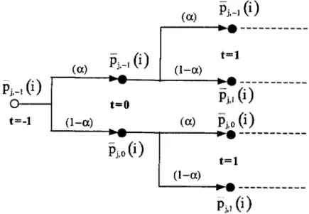
that maximize (29) given its demand equation (2). Note that such a

problem is separable into several independent simpler problems like (30), one for each branch

on the possibility tree depicted in Figure 4 of Appendix A.l regarding the event "the firm adjust its price in period

t,

once for good".

00

max Et

L

'YjaT-tQt,TTI (j5j,t (i), P;,T, }j,T, Wj,T (i); _￧ｾＩ＠

{Pi,t(i)} T t (30)

t ,(:) _ y;. (Pi,t(i))-(J

s.. Y),t - ),t Pi,t

Where TI (Pj,t (i), Pj,t, }j,t, Wj,t (i); ￧ｾＩ＠ represents TIj,t(i), according to its definition presented in (17).

Optimal solution implies:

E ｾ＠ 00 oT-tQ aTI j,t,T (') 'I,

I

=

O

t L.,; t,T

a- .

T=t Pj,t (1,) Pi,t{i)=Pj,t(i) (31)

Where TIj,t,T (i) = II (j5j,t (i), Pj,T, }j,T, Wj,T (i); ￧ｾＩ＠ and:

aTIj,t,T (i)

I

= (1 _ B) y;. [(Pj,t (i)) -(J _ y;. (Pj,t (i)) -(1+9).

ｾ＠

( ')]

a-o (i) J,T P. J..l J,T P. SJ,T 'I,

PJ,t

_.

p]' _' ｴＨｩＩ］ｰｾ＠ _], t(i) J,T J,T

Note that the optimal price pj,t (i) is a continuous function23 _{of o, e.g. pj,t (i)}

=

_{pj,t (o).}

Now we assess some properties ofthe firm's profit fiow value-function

lIj

(a), the profit fiow

function discounted at period t = O evaluated at the optimal prices {pj,t (a)} :0'

In the equilibrium analysis conducted in next section, we search for an equilibrium in which firms optimally decide a timeless24 _{price rigidity degree to be maintained in all periods, e.g.}

22 See the definition of the firm 's expected sum of profit fiow Ilj,t (i) in (17).

23Given the assumed regularity hypothesis regarding the functions at hand, the first order condition (31) implicitly defines an unique solution pj,t (í).

24Under such a timeless perspective, we mean that a particular firm has always chosen the same price stickiness degree D, and has always optimally behaved the same way, even before the initial period t = O. Such a time

firms decide on the stickiness degree before knowing the future realizations of random variables. Hence, such decisions must be based on unconditional expectations.

Note that the cost shock may lead to negative profits in some periods. Therefore, we

state the following assumption on the necessary condition of market existence, where Eçe TI; (a)

denotes the unconditional expected value, in

f"ê,

of TI; (a).

Assumption 11 If the firm i from Cj is present in the market then there exists a non-zero

probability measure for the households to choose this market, e.g. "Ij

>

O, and its unconditional expected profit fiow EçeTI; (-) is a continuous and non negative function of a.

Moreover, one easily conjectures that a particular firm maximizes TI; (a) when choosing a

flexible price strategy, e.g. a = O, for its expected profit "IjTIj,t (i) is maximized period-to-period

as previously shown in (17). Thus EçeTI; (-) is also optimized when a = O. Since higher values

of a imply in stronger restrictions25 _{to the fum's optimization problem (30), one expects that}

Eçe TI; (a) is a decreasing function of its argumento The following statement formalizes such a

conjecture:

Proposition 1 Under a timeless perspective, if a particular firm i is present in the market

then its expected profit Eçe TI; (a) is a decreasing function of the degree of nominal price rigidity summarized by the probability a.

The proof is given in Appendix A.2.

Corollary 1 If a particular firm i is present in the market then EçeTI; (O) ｾ＠ O.

The proof is straightforward once EçeTI; (O) ｾ＠ EçeII; (a), 'tia E [O,lJ.

We next assess the case in which the fum adopts the probability a of price stickiness, but

·when adjusting the fum decides instead for the sub-optimal price26 _{P;,t (Ci), where Ci ｾ＠ a.} Such a case is relevant, for we consider it when testing best responses in the further discussed equilibrium analysis.

In such a context, we define TIj (a, p* (Ci)) as the profit flow function of a fum that readjusts

with probability (1 _. a), discounted at period t = O and evaluated at the sub-optimal prices

{pj,t (Ci)}

:0'

where õi ｾ＠ a. Formally, TIj (a,p* (Ci)) satisfies:

IT: (a, p' (li» - Eo

t,

"rj [a'+lQo"IT (Pj,-di ), Pj", lj", Wj,' (i);

çi)

+

+

(1 - a)

t.

aT-'Qo,TIT

(pj,t

(li) , Pj,T, lj,T, Wj,T (i) ;

çi-) ]

(32) Now, we make the following statement:

Proposition 2 Under a timeless perspective, suppose that the i-th firm from Cj is present in

the market and adopts the probability a of price stickiness, but when adjusting it decides instead for the sub-optimal price P;,t (Ci), where Ci ｾ＠ a. In such a context the unconditional expectance of TIj (a, p* (Ci)), previously defined in (32), satisfies the following inequality:

25Since prices remain fi.xed for about 0:/ (1 - 0:) periods, on average, the restriction works almost as if higher values of o: "increased" the number of restrictions of the type "Pj,t (i) = pj,t-l (i)".

2ÜNote that pj,t (õ) would be the optimal price if the firm adjusted with probability (1 - õ) instead.

Eçerr1

(a:,p* (li)) ::;

Eçerr;

(li) for li

<

a: (33) The proof is given in Appendix A.3.

Therefore, a profit-maximizing fum that optimally readjust its price with probability (1 - õ)

have its expected profit decreased when increasing its price stickiness degree to o: 2: li even when readjusted prices are

{pj,t

(O:)};:o instead of

{pj,t

(li)}

;:0'

We next search for a particular equilibrium in which all firms of a particular consumption center endogenously choose the same time-invariant price stickiness degree. Such an equilibrium

.' is interesting for the standard literature assumes that all fums are identical regarding their

exogenously given nominal price rigidity degree, even if no adjusting costs apply. Our approach leads to an endogenous price stickiness degree as an optimal strategy of competing firms. We stress the fact that such a result follows from the traditionally assumed consumer risk aversion, so it applies even in an economy where firms have no adjusting costs.

2.3 The equilibrium

In line with the former assumption on distributions stationarity, we focus our analysis in search-ing for equilibrium outcomes in which agents' decisions are also time stationary regardsearch-ing the firms' choices on the degree of price stickiness. Although there should be other equilibria with

idiosyncratic time-varying parameter O:j,t (i), our choice for such a specific equilibrium simplifies

our analysis while still allowing for a broadening of the understanding of the sources of nominal rigidities. Moreover, such an equilibrium is in line with the basic standard approach in which the degree of nominal rigidity is time-invariant.

In order to simplify the argument, we may consider that a coalition is formed among all

the fums from each Cj , so that they all decide to adopt the same degree O:j of price stickiness.

Such coalition is formed for long-run reputation purposes, and its plausibility is only possible if there is a mechanism that penalizes each fum that refuses to adopt the group strategy. Indeed, consider the case in which no penalizing mechanism is created. Since every fum knows that its strategy has no infiuence over aggregate variables, they will choose the "free rider" fiexible price strategy, for it maximizes their individual profits. Thus the existence of such a coalition depends on the penalizing mechanism. However such a coalition strategy permits a competi tive advantage over the strategies adopted by the firms from the other consumption center, as will be shown further on. Therefore such a coalition assumption is not so strong. We abstract from issues concerning the coalition, such as the coalition central planner, and focus on its consequences.

Formalizing our arguments we define the equilibrium we search for:

Definition 4 The equilibrium of the above model economy consists on a set of dynamic

equa-tions characterizing the agents optimal behavior and a set of endogenously determined probability measures, such as the timeless degrees of nominal rigidity O:j adopted by each Cj, and also the timeless probabilities "fj of choosinrl7 the C_{j ,} both consistent with the agents solutions to their

inter-temporal maximization problem.

Note that the previous definition implies that all the fums, from the same Cj , that readjust

prices in period t choose the same optimal price

p;

(O:j). Note that the optimal price ultimately

regardless the consumption center they belong to. However, if the consumption centers adopt different degrees of price stickiness, e.g. in case of <lI ｾ＠ <l2, the readjusted prices will differ

from center to center. '

Thus the aggregate price Pj,t of each C_{j ,} defined in (3), may now be represented by the following expression.

1

P

[p

l-8 ( ) * ( )1-8] 1-8

j,t = <lj j,t-l

+

1 - <lj Pt <lj (34)

An interesting feature of our modelling assumptions is that once chosen the consumption center, everything tends to mimic the standard mo deIs in the literature, at least until the following period.

Before presenting the next proposition, which states that the representative household's

instantaneous utility function28 _{is concave in prices, we need some lemmas}29 _{regarding the}

following functions:

Pu IR++ -IR. (35)

Pu (x) - u [u

e

1 _(X1_/CI-8

»)]

Pv lR++-IR. (36)

Pv (x) , - V [f-I ＨｫｾＯｃｬＭＸＩＮ＠ u

e

1 (K X 1/ C1 - O

»))]

Where k

>

O and K

>

O.

Lemma 1 The previously defined function Pu (.) is strictly concave.

Lemma 2 lf the consumption utility function satisfies the following restriction30, e.g. if the

households are sufficiently prudent and risk averse, then the previously defined function Pv (.)

is strictly convexo

TJ (1.)

+

O (20 - 1) (J-l (1.)

>

30

(J;;1 (1.) r (37)

Where TJ (1.) = ｟ｵｾ｣｣｣ＨｾＩ＠

>

O is the Absolute Prudence lndex, _{ＨｊｾＱ＠} (1.) = - ｵｾ｣ｃｾＩ＠

>

O is the

Absolute Risk Aversion lndex and (J;1 (1.) = - ｵｾｾｩＺｪＧｾ＠

>

O is the Relative Risk Aversion lndex for 1.

>

O.

At a first glance the restriction (37) seems to be very strong. However in the case of the

widely used Constant Relative Risk Aversion (CRRA) utility functions31 , the parameters locus

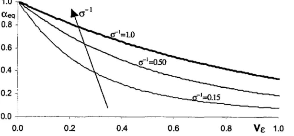
satisfying suc;h a restriction is quite wide. Note that the narrow gray area of Figure 1 indicates the region where (37) is not satisfied.

It is important to stress that such a restriction is just a necessary condition for the Lemma 2 to hold. The necessary and sufficient condition also includes labor disutility and production

28Remember that the instantaneous utility function considers both the consumption utility and the labor disutility, e.g. [u (Ct) - foI V (ht (i)) di] .

29Since their proofs are easy and purely algebraic, we omit them.

3°Its usual to consider the Absolute Prudence lndex in economic analysis in which agents make optimal choices in an inter-temporal decision environment with uncertainties. A good reference is Kimball (1990).

31For eRRA utility functions as u(c) = ｣ｬ［ｾＺｬｩｬＬ＠ with a constant relative risk aversion index 0-- 1 , the

absolute index of risk aversion and prudence are 0-;1 (c) = 0-- 1 jc and '" (c) = (1 + 0-- 1 ) jc, respectively.

So, the inequality (37) can be simplified to B (2B - 1) 0-- 2

+

(1 - 3B) 0-- 1 + 1 > O, whose solution set is: {0--1 E ]R : 0--1 <

2Ll

or 0--1 >

fi}·

o'

006 J ! 004

ｾ＠

I

02

j

000 -;-, - - - , - - - . - - , . - - - r - - , . - - - , - - - r - - - ,

2 3 4 5 6 7 8 9

e

1)

Figure 1: Convexity of P 1/ (.).

function parameters. Since its interpretation is less intuitive we did not present it. However such a new restriction narrows the gray area of Figure 1, making even wider the acceptance area where 1>1/ (-) is strictly convex in the case of the CRRA utility functions.

Now we are able to announce and prove an important proposition stating that a best response of the firms from one consumption center is to increase the degree of price stickiness relative to the one adopted by the firms from the other consumption centero

Proposition 3 Provided that restriction (37) is satisfied and that Eç-rri (O)

>

O, suppose that

the households always choose the C_1, e.g. "h

=

1 and "'12

=

00 Therefore, there is a small enough probability Q2

>

O such that if the firms from C₂ announce the following price setting

mechanism from a given period t onwards

C)

= { p; (O) , with probability (1 - Q2)

P2,t 1, P2,t-1 (i) , with probability Q2 (38)

then all households realize that they have better changing their strategies to

"'rI =

O and

1'2

=

1, benefiting the firms from C_{2 •}

The proof is given in Appendix A.4o

Based on the above arguments, we are able to formalize the characterization of the equilib-rium concept from the households' behavior standpoint, as the next theorem assesses.

Theorem 1 Provided that restriction (37) is satisfied and that Eç-rr; (O)

>

O, there is no

equi-librium in which the representative household always chooses the same consumption center32 •

Therefore, under such assumptions, households are indifferent between consumption centers in equilibriumo

The proof is given in Appendix A050

N ow, turning our attention to the firms behavior, the next theorem assess that firms choose

the equilibrium degree of nominal rigidity Qeq as the highest degree of price stickiness consistent

with a non-negative expected profit. Therefore such a theorem constitutes the key result of the present study.

Theorem 2 Provided that households are sufficiently prudent and risk averse, according to the

inequality (37) of above Lemma 2 and that Eç-rr; (O) 2': O, equilibrium requires that all firms

32There also won't be any equilibrium in which the representative household previously reveals his choice of

from both consumpti:on centers adopt the same highest degree of price stickiness QI

=

Q2

=

Qeq,

for which the expected profit is non-negative, e.g. EçeTI; (Qeq)

>

0, 't/j. Non-trivial solutions implies Eçdl; (Qeq) = 0, 't/j. Otherwise, if Eçdl; (1)

2:

°

then Qeq = 1 represents the trivial solution33 •

The proof is given in Appendix A.6.

Therefore, the above theorem implicitly defines the equilibrium stating that Eç-:TI; (Qeq) = 0,

't/ j in the non-trivial case.

Note that it has a Bertrand equilibrium flavor. However, instead of competition on prices per se as in the Bertrand case, the equilibrium at hand considers a competition on the parameter capturing the degree of price rigidity.

It is interesting to note that such a result follows from the two types of competition inputted in the model. The first one is the traditional monopolistic competition that allows each fum to choose an optimal price that maximizes its expected discounted profit flow. The second one is the contribution of our modelling assumption on consumption centers. Indeed in the first decision moment of each period

t,

households must decide from two "identical goods", namely the homogeneous consumption centers. Therefore, a oligopoly game must apply to model competition among both consumption centers. Since such a competition is conducted in terms of the degree of price stickiness, the Bertrand game captured the strategic behavior. As a consequence, the expected discounted profit flows turned to be zero in the non-trivial equilibrium, despite the fact they are the best furos can make optimally choosing their individual prices.

In order to dose this section three comments are in order. The first one concern the number of consumption centers in the model economy. In spite of adopting only two centers in the above economy, the obtained results can be easily extended to a larger number of consumption centers.

The second one refers to the fact that the above theorem generalizes the perfect competi tive equilibrium result of zero profits. Theorem 2 states that such a profit is zero on average or in expected terroso

The third one is based on Proposition 3. The uncertainty regarding the exogenous shock

êt, which does notaffect the households' preferences neither the furos' productivity, make

households postpone the flexible prices environment.

Such a result is achieved from the fact that the expected utility decreases with the uncer-tainty regarding the flexible prices environment. We showed that a sticky price environment, at least a Calvo's type one, is preferred to the one with flexible prices. However it is important to point out that we did not proved that households prefer the Calvo's type nominal rigid-ity the mosto It is possible that other price filtering procedures may also reduce the implied uncertainty, but such a study does not belong to the scope of the present analysis.

Note that EE,e TI; (Qeq) depends on the distribution of TI (p; (Qeq) , Pj,t, Yj,t, Wt (i) ;

çD,

so the

non-trivial equilibrium condition

Eçerr;

(Qeq) =

°

implies that he endogenous degree of price stickiness Qeq depends on the distributions of aggregate price and production. But such distri-butions surely depend on the way monetary policy is conducted, for it determines the expected path of aggregate variables. Therefore the Lucas' critique may be applied, for changes on the way monetary policy is conducted may lead to changes in the endogenous degree of price stickiness and in the coefficients of structural equations.

Moreover, we expect that the equilibrium price rigidity would depend on the distribution of the exogenous shock, so structural breaks in the stochastic process of êt affect Qeq.

Therefore, we could extend the concept behind the Lucas' critique. The dependency of the degree of price rigidity on the distribution of the exogenous cost shock strongly suggests that

33Note that if EçeIIj (1) < 0, 'ij then there is no equilibrium, for there are no firms in the market.

..

the traditional monetary policy evaluation exercises using macroeconometric models could be fiawed. Typically estimated relations, even with quasi-structural equations, containing future expectations derived with an ad hoc imposed nominal rigidity source, are reduced-form rather than truly structural relations, for structural changes in the stochastic process generating the cost shocks can change the optimal degree of price stickiness chosen by the firms.

Therefore, as a policy-oriented implication of the present study we recommend the utilization of econometric models with time-varying parameters in order to assess possible parameters structural breaks even if the implemented policy remains unchanged.

In the following section, we introduce the model's first and second order approximations for the corresponding structural equations. Among other results, we show that: (a) the degree of inefficiency cP_y constitutes a source of nominal price rigidity; and (b) the equilibrium (optimal) degree of price rigidity aeq depends on the coefficient of variation of the random shock êt, for

a given monetary policy rule.

3

Log-approximated structural equations

Initially, it is convenient to derive log-approximations for aggregate product and prices through the consumption centers, adopting the following notation as the percentage deviation of each variable from its steady state value. For any variable Xt, always positive or negative, with a

steady state value

x,

we define Xt

=

log (xt/

x).

It is easy to verify that the expressions (4) and (6) imply the following first order Taylor approximations:

Yt

-

"Yí,t

+

(1 -,,)

Y2,t

P

t

-

"Pl,t

+

(1 - ,,)

P

2

,t

(39)

(40)

Moreover, from (24) and (26), we log-linearize the natural and the efficient34 _{products as}

follows:

(41) (42)

Where cPy is the previously defined inefficiency degree parameter and " denotes the

time-invariant probability of choosing the C1 , e.g. " = "1.

Assuming that the distribution support of êt is completely inside ｾＫ＠ or lR_, we obtain the

following log-linearizations for the real marginal cost:

- fL

(1-

cPy)

(w

+

a-I)

Y;,t

+

fLE Êt

s/

-

fL

(1 -

cPy)

(w

+

a-I)

Yt

+

fLE €t (43)

Wh _ere ... e I ( e) Sy (V,v) Y -1 ucc (V) Y· h d I ' . k

SJ" _, t

=

og fLSJ" _, t , W

= ( )

_{s Y,Y} ,a

= - ()

_{Uc Y} IS t e stea y state re atlve rIS

aversion index, and

s/

=

Ｂｓｉｾｴ＠

+

(1 - ,,) ｓＲｾｴ＠ aggregates the real marginal costs from each consumption center.

34If 1>y is dose enough to zero, the approximated log-deviation of the efficient production from the steady