www.atmos-chem-phys.net/15/10581/2015/ doi:10.5194/acp-15-10581-2015
© Author(s) 2015. CC Attribution 3.0 License.
Use of North American and European air quality networks to
evaluate global chemistry–climate modeling of surface ozone
J. L. Schnell1, M. J. Prather1, B. Josse2, V. Naik3, L. W. Horowitz4, P. Cameron-Smith5, D. Bergmann5, G. Zeng6, D. A. Plummer7, K. Sudo8,9, T. Nagashima10, D. T. Shindell11, G. Faluvegi12, and S. A. Strode13,14
1Department of Earth System Science, University of California, Irvine, CA, USA
2GAME/CNRM, Météo-France, CNRS – Centre National de Recherches Météorologiques, Toulouse, France 3UCAR/NOAA Geophysical Fluid Dynamics Laboratory, National Oceanic and Atmospheric Administration,
Princeton, NJ, USA
4Geophysical Fluid Dynamics Laboratory, National Oceanic and Atmospheric Administration, Princeton, NJ, USA 5Lawrence Livermore National Laboratory, Livermore, CA, USA
6National Institute of Water and Atmospheric Research, Lauder, New Zealand
7Canadian Centre for Climate Modeling and Analysis, Environment Canada, Victoria, British Columbia, Canada 8Department of Earth and Environmental Science, Graduate School of Environmental Studies, Nagoya
University, Nagoya, Japan
9Department of Environmental Geochemical Cycle Research, Japan Agency for Marine-Earth Science and Technology,
Yokohama, Japan
10Center for Regional Environmental Research, National Institute for Environmental Studies, Tsukuba, Japan 11Nicholas School of the Environment, Duke University, Durham, NC, USA
12NASA Goddard Institute for Space Studies, and Columbia Earth Institute, Columbia University, New York, NY, USA 13NASA Goddard Space Flight Center, Greenbelt, MD, USA
14Universities Space Research Association, Columbia, MD, USA
Correspondence to:J. L. Schnell (jschnell@uci.edu)
Received: 16 February 2015 – Published in Atmos. Chem. Phys. Discuss.: 16 April 2015 Revised: 9 September 2015 – Accepted: 9 September 2015 – Published: 25 September 2015
Abstract. We test the current generation of global chemistry–climate models in their ability to simulate ob-served, present-day surface ozone. Models are evaluated against hourly surface ozone from 4217 stations in North America and Europe that are averaged over 1◦×1◦ grid cells, allowing commensurate model–measurement compari-son. Models are generally biased high during all hours of the day and in all regions. Most models simulate the shape of re-gional summertime diurnal and annual cycles well, correctly matching the timing of hourly (∼15:00 local time (LT)) and monthly (mid-June) peak surface ozone abundance. The am-plitude of these cycles is less successfully matched. The ob-served summertime diurnal range (∼25 ppb) is underesti-mated in all regions by about 7 ppb, and the observed sea-sonal range (∼21 ppb) is underestimated by about 5 ppb ex-cept in the most polluted regions, where it is overestimated
1 Introduction
We test simulated present-day surface ozone in global chemistry–climate models on temporal scales from diurnal to multi-year variability and on statistics from median geo-graphic patterns to the timing and size of extreme air quality episodes. The tests use gridded hourly surface ozone abun-dances based on a decade of observations from 4217 air quality monitoring sites in North America (NA) and Europe (EU). Chemistry-climate models provide a valuable means for projecting future air quality in a changing climate (Kirt-man et al., 2013), but recent assessments have lacked com-mensurate observational comparisons to establish their cred-ibility in reproducing current cycles of surface ozone over polluted regions (Young et al., 2013). Model–measurement comparisons to date have identified model faults, yet they have often been limited to monthly statistics, biased to pick-ing clean-air sites over limited parts of the continents (Fiore et al., 2009; Doherty et al., 2013), and avoided evaluating diurnal cycles and the patterns of major pollution episodes (Schnell et al., 2014, henceforth S2014).
The factors driving future surface ozone (O3) changes
in-clude (1) local-to-regional emissions, (2) global-scale emis-sions of air pollution transported across continents and oceans, (3) global emissions and physical climate change that alters the hemispheric-scale abundances of tropospheric O3, and (4) climatic shifts in the meteorology that creates the
worst pollution episodes. Factors (1), (2), and (3) have been studied extensively with global chemical transport models (CTMs) and chemistry–climate models (CCMs), and there is some agreement on model projections given an emissions scenario (e.g., Prather et al., 2003; Reidmiller et al., 2009; HTAP, 2010; Wild et al, 2012; Doherty et al., 2013; Young et al., 2013). The importance of (4), however, lies in the recog-nition that air quality extremes (AQX), the worst pollution episodes in a decade, are triggered by meteorological condi-tions. Air quality absolute exceedances are known to occur in multi-day, spatially extensive episodes over the USA (Logan, 1989; Seinfeld et al., 1991), but it was not until the regular gridding of all station data over North America and Europe and the statistical definition of extremes in S2014 that the extent, coherence, and decadal variability of the episodes be-came clear. If climate change increases the duration and/or extent of the worst decadal AQX episodes, then the over-all health impact of poor air quality may be worse than ex-pected based on precursor emission changes alone (Fiore et al., 2012). A warming climate appears to increase the num-ber of stagnation days (Horton et al., 2014) and may decrease the frequency of ventilating midlatitude cyclones (e.g., Mick-ley et al., 2004), but it is unclear how these meteorologi-cal indices relate to surface O3or particulate matter,
espe-cially with respect to the worst AQX episodes as identified in S2014.
The models in the Atmospheric Chemistry and Climate Model Intercomparison Project (ACCMIP; Lamarque et al.,
2013) were used in the recent assessment of the Intergov-ernmental Panel on Climate Change (IPCC; Kirtman et al., 2013) and represent the most advanced attempt to simulate global surface O3in a future climate. However, in order to
place any confidence in their projections, their ability to sim-ulate the observed, present-day surface O3climatology must
be evaluated. In this paper we present the first such model– measurement comparisons, specifically addressing (4) by ap-plying the methodologies from S2014 to the current genera-tion of CCMs in an effort to quantify their ability to simu-late the decadal statistics of the AQX episodes. Due to the complexity and nonlinearity of the underlying processes, ac-curately simulating surface O3over both clean and polluted
environments is a formidable task for global models with res-olutions of 100 km at best. For example, it has been shown that choices in the parameterization of surface deposition can shift modeled surface O3levels by 10 ppb or more (Val
Mar-tin et al., 2014). Moreover, there are new, phenologically based land-surface models for interactions between atmo-spheric chemistry and the biosphere (Büeker et al., 2012) that have yet to be fully implemented in global models. In any case, both recent and future land-use change is expected to impact surface O3 abundances (Ganzeveld et al., 2010).
Thus, we recognize that this model–measurement compari-son is just one of the first steps in evaluating global model simulations of surface O3pollution. A summary of the
ob-servational and model data sets as well as a brief overview of the methods developed in S2014, and used here, is presented in Sect. 2. Model–measurement comparisons are presented in Sect. 3 with concluding remarks and further discussion in Sect. 4.
2 Data and methods
2.1 Observations of surface O3
We use 10 years (2000–2009) of hourly surface O3
mea-surements from air quality networks in NA and EU. Fol-lowing S2014, in NA we use 1633 stations from the US Environmental Protection Agency’s (EPA) Air Quality Sys-tem (AQS) and also increase the spatial coverage in NA by including 92 stations from the US EPA’s Clean Air Status and Trends Network (CASTNet) and 207 stations from En-vironment Canada’s National Air Pollution Surveillance Pro-gram (NAPS). The data sets used for EU remain the same as S2014: 2123 stations from the European Environment Agency’s air quality database (AirBase) and 162 stations from the European Monitoring and Evaluation Programme (EMEP; Hjellbrekke et al., 2013). Table 1 provides a sum-mary of the observational data sets.
A major advance by S2014 was the generation of aver-age surface O3abundance in a grid cell from observational
gen-Table 1.Observational data sets (2000 to 2009).
Domain Surface ozone network No. stations URL or reference
North US EPA Air Quality System (AQS) 1633 http://www.epa.gov/ttn/airs/aqsdatamart
America (NA) US EPA Clean Air Status and Trends
Network (CASTNet)
92 http://epa.gov/castnet/javaweb/index.html
Environment Canada’s National Air Pollution Surveillance Program (NAPS)
207 http://maps-cartes.ec.gc.ca/rnspa-naps/data.aspx?lang=en
Europe (EU) European Monitoring and Evaluation
Programme (EMEP)
162 Hjellbrekke et al. (2013)
European Environment Agency’s air quality database (AirBase)
2123 www.eea.europa.eu/data-and-maps/data/
Table 2.Model summary.
(Abbreviation) model Modeling center Member∗ Resolution (lat.×lon) No. years Reference(s)
(A) MOCAGE MeteoFrance r2i1p1, v2 2◦×2◦ 4 Josse et al. (2004)
Teyssèdre et al. (2007)
(B) GFDL-AM3 GFDL r1i1p1, v2 2◦×2.5◦ 10 Donner et al. (2011)
Naik et al. (2013)
(C) CESM-CAM-SF LLNL-NCAR r1i1p1, v4 ∼1.9◦×2.5◦ 10 Cameron-Smith et al. (2006)
Lamarque et al. (2013)
(D) UM-CAM NIWA r1i1p1, v2 2.5◦×3.75◦ 10 Zeng et al. (2008, 2010)
(E) CMAM CCCma r1i1p1, v2 ∼3.7◦×3.75◦ 10 Scinocca et al. (2008)
(F) MIROC-CHEM JAMSTEC-NU-NIES r1i1p1, v2 ∼2.8◦×2.8125◦ 10 Watanabe et al. (2011)
(G) GISS-E2-R GISS r1i1p3, v1 2◦×2.5◦ 5 Koch et al. (2006)
Shindell et al. (2013)
(H) GEOSCCM NASA-GSFC r1i1p1, v1 2◦×2.5◦ 10 Oman et al. (2011)
(I) UCI CTM UCI – ∼2.8◦×2.8125◦ 10 Holmes et al. (2013)
∗The formatr<N>i<M>p<L>, vX distinguishes among closely related simulations by a single model where the set of integers (N, M, L, X) formatted as shown (e.g.,
r2i1p1, v2) define each model simulation’s realization number (N), initialization method (M), perturbed physics version (L), and version of publication-level data set (X).
erate a 1◦×1◦ hourly grid-cell average surface O3
prod-uct over NA and EU using the interpolation scheme de-scribed in S2014. The interpolation is similar to an inverse distance-weighted interpolation but additionally incorporates a declustering technique employed to reduce data redun-dancy, similar to that of Kriging (Wackernagel, 2003). The method also avoids disproportionately representing stations that often are preferentially placed in the most polluted ur-ban environments. S2014 first derived the maximum daily 8 h averages (MDA8) of the individual stations and then in-terpolated onto the 1◦×1◦ grid, while here we interpolate the hourly measurements and subsequently derive the MDA8 at each grid cell. Differences between the two methods are small (e.g., some missing station data, different 8 h periods for nearby stations), but the new approach allows modeled di-urnal cycles to be analyzed. The effects of (i) the new hourly 1◦×1◦cells being used to calculate MDA8 and (ii) the ad-dition of CASTNet and NAPS stations on the decadal 25th, 50th, and 95th percentiles at each grid cell in NA are shown in Fig. S1 in the Supplement. Overall, the difference (this work minus S2014) is about−0.6 parts per billion (ppb) O3
for each of the three percentiles. These decreases are most likely a result of deriving MDA8 from the interpolated hourly abundances rather than first deriving each station’s MDA8 and then interpolating. Other notable changes are the north-east edge of the domain (−5 ppb) for all three percentiles due to the generally lower O3 abundances of Canadian NAPS
stations, and Wyoming and Colorado at the 25th percentile (+5 ppb) possibly from CASTNet stations, reflecting either cumulative production of O3as polluted air reaches them or
else more prevalent stratospheric influx.
2.2 Description of models (ACCMIP+UCI CTM) The ACCMIP consists of 16 global models (12 CCMs, two CTMs, and two chemistry general circulation models, CGCMs) and was designed with the intent to better under-stand the relationships between atmospheric chemistry and climate change (Lamarque et al., 2013). We focus on the
ac-chistexperiment, designed to test the models’ ability to
one CGCM) with archived hourly surface O3, incorporating
the years from each model most closely aligned with obser-vations. Most models provide 10 years of data, starting in either model year 2000 or 2001. In any case, all ACCMIP simulations are climatologically representative of the aver-age 2000s with respect to meteorology and emissions. Ta-ble 2 provides a brief summary and the references of the models used in this study. Detailed descriptions of the AC-CMIP models can be found in Lamarque et al. (2013) and references therein.
We also include a hindcast simulation over the same pe-riod as the observations from the University of California Irvine Chemical Transport Model (UCI CTM) performed at T42L60 resolution (Holmes et al., 2013) to both compare our model with the current generation models and to highlight differences between model simulations using free-running and hindcast meteorological conditions. The UCI CTM had many updates since the 1◦×1◦×L40 version (Tang and
Prather, 2010) used by S2014, but calculates similar, not un-expectedly high-biased patterns of surface O3.
For commensurate comparison of the models and mea-surements, we regrid the modeled hourly O3 abundances
(typically at 2 to 3◦resolution) to the same 1◦×1◦cells as the observations using first-order conservative mapping (i.e., proportion of overlapping grid-cell areas). Modeled hourly abundances are adjusted by 1 h per 15◦longitude to be con-sistent with the local time of the observations. Our two major domains are NA bounded by 25–49◦N and 125–67◦W and EU bounded by 36–71◦N and 11◦W–34◦E. A further mask-ing drops coastal grid cells for which the quality of predic-tion index,QP< 2/3 (the number of independent stations at an effective distance of 100 km used to calculate the grid-cell values), see S2014 and Fig. S2 in the Supplement. Table S1 in the Supplement provides the latitudes and longitudes used in the final masking for both domains. Because of their dif-fering chemical regimes, some of our analyses split the NA domain into western (WNA) and eastern (ENA) regions at 96◦W, and EU into southern (SEU) and northern (NEU) re-gions at 53◦N.
2.3 Air quality extremes
We define AQX events on a daily basis using local (i.e., grid-cell) climatologies to identify the 10 times N worst days (i.e., highest MDA8) in an N-year period (i.e., the ∼97.3 per-centile; e.g., the 100 worst days in a decade). The space–time connectedness of the AQX events into episodes is defined using a hierarchal clustering algorithm described in S2014. Because AQX episodes span across the regions, statistics for these analyses are done only on the two major domains NA and EU. The total size of an AQX episode (S, units
=km2days) is calculated by integrating the areal extent of an episode (km2) through time (days). For a given set of episodes, the mean size (S) is calculated as a weighted ge-ometric mean, with the weights equal to the AQX episode
sizes (Eq. 6 in S2014). Because the lower native resolutions of the models typically map onto four to eight contiguous 1◦×1◦grid cells, the modeled episode sizes have artificial
minima; however, S2014 demonstrated that this has little ef-fect on the resultant episode size distributions.
3 Results
3.1 Diurnal cycles
We test the models’ abilities to reproduce the observed shape (i.e., phase and amplitude) of the diurnal cycle, averaged over summer (JJA) and winter (DJF) months. For each of the four regions, average hourly values (local solar time) are calcu-lated as the area-weighted mean of all grid cells’ O3
abun-dances. We calculate the phase (h, hour of peak O3
abun-dance, withh= 0.0 corresponding to 00:00 LT) and peak-to-peak amplitude (H, ppb difference from minimum to max-imum) of the diurnal cycle using a cosine fit with a period of 24 h. Although the diurnal cycle could be more accurately represented by a higher-order fit, this simple method provides objective and continuous measures ofhandH for each data set, avoiding subjective, ambiguous results in cases of flat and/or multiple maxima.
Figure 1a–h show the diurnal cycle of the observations and models averaged over JJA (top row) and DJF (second row) in WNA, ENA, SEU, and NEU (columns from left to right). A triangle for each data set is plotted as (x,y)=(h,H). The large number of data points (∼106×24 h per model)
pro-vides a smooth and robust estimate of each data set’s diur-nal cycle. The color scheme and model abbreviations in the legend of Fig. 1 are common to all similar figures and text throughout. The Taylor diagrams (Taylor, 2001) in Fig. S3a– h in the Supplement show an alternate, commonly used sum-mary of the results in terms of the correlation coefficient (R), the normalized standard deviation (NSD), and centered root-mean-square difference. Figures 1 and S3 in the Supplement show very similar quantities (e.g., model–measurement dis-crepancies inhandHroughly correspond toRand NSD, re-spectively); however, we consider the representation in Fig. 1 to be more useful. The panels of Fig. S3 in the Supplement correspond to panels in Fig. 1 in terms of region and vari-able. Summary statistics on diurnal cycles, annual cycles, and AQX events for ENA are presented in Table 3, with all re-gions and additional statistics provided in Tables S2–S4 in the Supplement.
The shape of the diurnal cycle of O3 is driven primarily
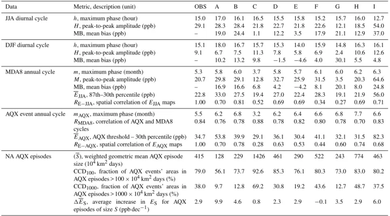
Table 3.Example summary statistics for the observations (OBS), the ACCMIP models (A–H), and the UCI CTM (I) for eastern North American (ENA) summer (JJA) and winter (DJF) diurnal cycles, annual cycle of MDA8, annual cycle of AQX events, and North American (NA, combined western North America (WNA) and ENA) AQX episodes (100 AQX events per decade case).
Data Metric, description (unit) OBS A B C D E F G H I
JJA diurnal cycle h, maximum phase (hour) 15.0 17.0 16.1 16.5 15.5 15.8 15.2 15.7 16.0 12.7 H, peak-to-peak amplitude (ppb) 29.1 28.3 28.4 21.8 22.7 21.8 22.6 12.1 18.5 54.0
MB, mean bias (ppb) – 19.0 24.4 1.1 12.2 3.5 17.9 21.1 12.9 37.0
DJF diurnal cycle h, maximum phase (hour) 15.1 18.0 16.7 15.7 15.3 14.0 15.9 14.8 16.3 16.1 H, peak-to-peak amplitude (ppb) 9.1 6.7 7.5 11.3 7.8 5.8 6.9 2.4 10.6 12.6
MB, mean bias (ppb) – 10.2 13.2 9.8 −1.5 −4.6 4.0 30.1 5.5 4.8
MDA8 annual cycle m, maximum phase (month) 5.3 5.8 6.0 3.7 5.8 5.7 6.1 6.0 6.2 6.3
M, peak-to-peak amplitude (ppb) 20.7 29.8 29.1 12.8 32.7 25.9 31.5 3.5 20.3 64.6
MB, mean bias (ppb) – 16.9 16.6 6.8 4.2 −4.2 8.1 20.1 8.0 24.8
EJJA, 87th–30th percentile (ppb) 22.8 33.0 27.5 19.4 27.0 22.4 28.3 19.1 21.9 56.0 RE−JJA, spatial correlation ofEJJAmaps 1.00 0.70 0.81 0.52 0.69 0.69 0.34 0.27 0.69 0.71 AQX event annual cycle mAQX, maximum phase (month) 5.5 6.2 6.8 3.2 6.2 6.4 6.6 6.8 7.7 6.6
RMDA8, correlation of AQX and MDA8 cycles
0.84 0.76 0.78 0.88 0.78 0.82 0.80 0.78 0.70 0.83 EAQX, AQX threshold – 30th percentile (ppb) 34.7 53.8 39.9 29.1 36.1 30.4 41.1 32.1 31.5 82.3 RE−AQX, spatial correlation ofEAQXmaps 1.00 0.70 0.78 0.28 0.63 0.53 0.44 0.60 0.74 0.68 NA AQX episodes (S), weighted geometric mean AQX episode
size (104km2days)
415 128 229 1426 461 290 522 243 774 463
CCD100, fraction of AQX events’ areas in AQX episodes > 100×104km2days (%)
79.0 56.1 73.7 92.6 85.3 76.1 80.3 73.0 83.0 80.2 CCD1000, fraction of AQX events’ areas in
AQX episodes > 1000×104km2days (%)
38.0 9.7 12.8 69.2 30.8 19.2 43.6 12.7 48.7 37.5
1ES, average increase in ES for AQX episodes of sizeS(ppb dec−1)
2.9 9.9 4.6 0.8 2.3 2.9 −0.1 3.5 2.9 6.0
is no obvious diurnal cycle in observations and the double minimum may simply reflect the titration of O3 from the
morning and afternoon peaks in transport NOx emissions.
In this case there is little information from the diurnal cycle except that the amplitudeHis small. The ACCMIP models, but not the UCI CTM, mostly showhwithin±1 h, generally later than observed (Tables 3 and S2 in the Supplement).
Although the ACCMIP models’ diurnal phase closely matches the observed, the peak-to-peak amplitudeH is less successfully simulated. For JJA the observed H is 27, 29, 24, and 14 ppb in WNA, ENA, SEU, and NEU, respectively; for DJF, H is 10, 9, 5, and 0.2 ppb. We characterize the three largestH’s as high-photochemical region-seasons (JJA in WNA, ENA, and SEU) and the remaining five as low-photochemical. In this sense JJA in NEU is closer to DJF in ENA in terms of near-surface O3 production. The
AC-CMIP models generally underestimateH by about 7 ppb in the highest three region-seasons but cluster aroundHfor the lowest five. Model A is the only ACCMIP model to over-estimateH in any of the highest three, possibly as a result of its large total VOC (volatile organic compounds, exclud-ing methane) emissions (55 % larger than the average of the other seven models). The 24 h mean bias (MB, see Tables 3 and S2 in the Supplement) for the ACCMIP models is typ-ically positive in all eight region-seasons (up to 28 ppb), al-though some models (e.g., C and E in JJA, E in DJF) show
little or no mean bias, even though they underestimateHin JJA by about 25 % like all ACCMIP models.
The underestimation of the summertime diurnal amplitude H by most ACCMIP models suggests that they either un-derestimate net daytime production or have too little night-time loss of O3or its precursors through either in situ
chem-ical loss or dry deposition. From the derivative of the di-urnal cycles in Fig. 1a–d, there are two periods of model– observation discrepancy: in the early morning (∼06:00 LT) models underestimate the observed slope and in the early evening (∼19:00 LT) they overestimate it. The models gen-erally match the observed slope to within±1 % h−1during midday and throughout the night. Thus the model error is to underestimate net O3 production in the early morning and
overestimate it in early evening, which may be caused by the lack of a diurnal emission cycle in these global models. The mismatch of the slope in the early morning, during which the boundary layer grows rapidly, may be caused by the models underestimating entrainment of free troposphere air. We find no clear evidence that modeling errors in the nocturnal plane-tary boundary layer (Lin et al., 2008) or missing near-surface processes affect the diurnal cycle on a regional average.
0 10 20 30 40 50 60 70 80 90 100 a)
Summer (JJA) O
3
abundance (ppb)
0 3 6 9 12 15 18 21 24 0 10 20 30 40 50 60
WNA (local time, hr)
e)
Winter (DJF) O
3
abundance (ppb)
b)
0 3 6 9 12 15 18 21 24
ENA (local time, hr)
f) c)
0 3 6 9 12 15 18 21 24
SEU (local time, hr)
g) 0 10 20 30 40 50 60 70 80 90 100 d)
0 3 6 9 12 15 18 21 24 0 10 20 30 40 50 60
NEU (local time, hr)
h) 0 10 20 30 40 50 60 70 80 90 100
Mean MDA8 O
3
(ppb)
i)
J F M A M J J A S O N D J 0 10 20 30 40 50 60 70 WNA (month)
AQX events (%)
m)
j)
J F M A M J J A S O N D J
ENA (month)
n)
k)
J F M A M J J A S O N D J
SEU (month) o) 0 10 20 30 40 50 60 70 80 90 100 l)
J F M A M J J A S O N D J 0 10 20 30 40 50 60 70 NEU (month) p)
O Observations A MOCAGE B GFDL−AM3 C CESM−CAM−SF D UM−CAM
E CMAM F MIROC−CHEM G GISS−E2−R H GEOSCCM I UCI CTM
Figure 1. (a–h)Diurnal cycles of hourly O3abundances (ppb) for the observations (O), ACCMIP models (A–H), and UCI CTM (I) averaged
over (a–d)summer (JJA) and(e–h)winter (DJF) months in (a,e) WNA, (b, f) ENA, (c, g) SEU, and (d,h) NEU. Triangles show the
observation’s and models’ cosine fit derived values of the hour of maximum phasehand peak-to-peak amplitudeH plotted as (x,y)=(h, H) for each season, region, observation, and model. (i-p) Annual cycles of (i–l) MDA8 O3and (m–p) AQX events in (i,m) WNA, (j,n)
ENA, (k,o) SEU, and (l,p) NEU. The filled gray curve shows±1σfor each month (calculated across years) for the observations. Triangles show the observations’ and models’ cosine fit derived values of the MDA8 cycle month of maximum phasemand peak-to-peak amplitude Mplotted as (x,y)=(m,M) for each region, observation, and model.
all the ACCMIP models in addition having the largest VOC emissions, is one of the few models to consistently overesti-mateH. In contrast, C and E are two of the better-performing models despite their comparatively simple representation of VOC chemistry (C – only isoprene, E – none). The only mod-els to include the small and relatively uncertain fractional yield of HNO3from the reaction of HO2and NO are A, G,
and H (Lamarque et al., 2013). This reduces daytime produc-tion and could partly explain why the models G and H con-sistently underestimateHmore than others, however model A overestimatesH.
The ACCMIP models reproduce the phase of the observed diurnal cycle in both seasons despite not accounting for hourly variation in emissions. The weekly emission-driven cycles in MDA8 O3 were diagnosed by S2014, but we do
not apply that diagnostic here because the models did not in-clude such variability in emissions. The lack of hourly varia-tion of emissions may account for the overall underestimates ofH by the ACCMIP models, since NO emissions can be lost heterogeneously at night, less effectively than those dur-ing the morndur-ing and afternoon peaks in traffic. In addition, if the early morning peak in transport NOxemission was
be augmented, thus yielding larger values of H. The AC-CMIP models use a wide range of boundary layer mixing schemes but consistently underestimate H. The boundary layer schemes may be responsible for these underestimates; however, Menut et al. (2013) notes that at least for one model, increasing its vertical resolution results in very small surface O3changes.
The UCI CTM’s values ofhandHshow that it drastically overestimates net daytime O3production, especially during
early morning hours. Its values ofh are about 2.4 h earlier than observed in the highest three region-seasons, and in con-trast to the ACCMIP models itsHvalues are too large by 10 s of ppb. This diagnostic identifies a serious problem with the UCI CTM diurnal cycle over polluted regions that needs to be investigated (e.g., missing heterogeneous loss of NO2at
night, capped boundary layer in the morning) and which will be done after publication of this research. S2014 found that the UCI CTM accurately hindcast the summertime probabil-ity distribution of MDA8 O3, the occurrence of AQX events,
and the size of these episodes, albeit with high bias of about
+29 ppb in JJA over both NA and EU. This new diurnal di-agnostic has clearly identified model errors and pathways to improve our model as well as models like G, which gravely underpredicts the amplitude of the diurnal cycle. The tests shown here emphasize a large-scale average over different photochemical regimes in the four regions, and thus individ-ual model developers may wish to analyze the observations for smaller regions using the data sets generated here, which are available by request from the corresponding author.
3.2 Annual cycle
We test the models’ abilities to reproduce the observed phase and amplitude of the annual cycle over the four regions. Av-erage monthly values for each region are calculated as the area-weighted mean of all encompassed cells’ MDA8 O3
abundance, reflecting the EPA air quality metric (www.epa. gov/air/criteria.html). Similar to the diurnal cycle, we derive the phase (m, month of peak O3 abundance, with m=0.0
corresponding to 1 January) and peak-to-peak amplitude (M, ppb difference from minimum to maximum) using a cosine fit assuming 12 equally spaced monthly means. Figure 1i–l show the annual cycle of the observations and models over our four regions with triangles plotted for each model and data set as (x,y)=(m,M). The filled gray curve shows±1 standard deviation of each monthly mean based on 10 years of observations. This interannual variability is quite narrow, much less than the spread across models. As for the diurnal cycle, the Taylor diagrams in Fig. S3i–l show an alternate presentation of the annual cycle results with summary statis-tics given in Tables 3 and S3 in the Supplement.
In northern midlatitudes, processes that drive the shape of the annual cycle are similar to those of the diurnal cy-cle (i.e., sunlight, temperature, and precursor emissions) but occur on continental to hemispheric scales. Dry deposition
through stomatal uptake and large-scale meteorological con-ditions including stratosphere–troposphere exchange and the position of the jet stream (Barnes and Fiore, 2013) also play important roles. These surface observations show the same well-known cycle that has been seen in the northern hemispheric midlatitude troposphere from ozone sondes and clean-air remote sites (Logan, 1989; Fiore et al., 2009): low-est values in late fall (ND), increasing through winter (JFM) followed by a broad flat peak over spring–summer (AMJJA). The lower reactivity region NEU peaks in April and declines until January, indicating meteorologically driven increases through the winter (e.g., stratospheric influx). The observa-tions show a phasem=5.6, 5.3, 5.5, and 4.3 month of year for WNA, ENA, SEU, and NEU, respectively; and corre-sponding amplitudesM=22, 21, 26, and 17 ppb. By fitting a cosine curve to each grid cell’s time series, we find that in terms of specific locations, the earliestmoccur in Canada, Florida, and NEU while the latest m occur in California, south-central NA, and SEU (not shown). Most ACCMIP models havemwithin±1 month of the observations, gener-ally earlier in NEU, later in ENA and SEU, and split in WNA. Models C and G have difficulty producing the observed sea-sonal cycles, and their derived phases are not meaningful.
The amplitudeMis controlled by both meteorology and photochemistry. For the very large regional values ofM, it is clearly chemical, occurring in regions with large O3
pre-cursor emissions: California with∼40 ppb, the Great Lakes region with∼30 ppb, and northern Italy with∼45 ppb (not shown). The smallest values ofM (∼15 ppb) are found in northwest and southeast NA and in NEU. The ACCMIP models generally underestimateMby about 5 ppb in WNA, SEU, and NEU, while they overestimate it by about 5 ppb in ENA. The low values ofMfor C and G suggest they are either overestimating net production of O3in winter or
un-derestimating it in summer; however, their wintertime biases (see Fig. 1e–h, Tables 3 and S2 in the Supplement) indicate that wintertime production or representation of wintertime physical climate could be causing the lowMvalues.
The annual cycles here are constructed using the MDA8 O3derived from hourly data. Many models, including eight
other ACCMIP models not analyzed here, do not report hourly surface O3 but only monthly means (i.e., the
13, and 9 ppb. This result was expected since the ACCMIP model ensemble generally has the largest biases outside of MDA8 hours. These conclusions are generally true for all seasons and models, as illustrated in Fig. S4 in the Supple-ment, which shows the mean bias (model minus observed) of MDA8 minus 24 h average for each model, season, and region.
For the UCI model, excess production in the diurnal cycle is also evident in the annual cycle, overestimating Min all regions, most in ENA (+44 ppb) and least in NEU (+9 ppb). In addition, the month of peak abundance is always later than observed, sometimes by more than 1 month. Not un-expectedly, the bias inMusing 24 h averages is significantly less than that using MDA8 (e.g.,+30 vs.+44 ppb in ENA) because the largest errors occur near midday. We conclude that using 24 h averages to construct the annual cycle is ba-sically a different, almost independent diagnostic than that constructed from the daily MDA8 O3, and further it would
predict different health impacts if used to project summer-time surface O3in a future climate.
3.3 AQX events
Next, we test the models’ ability to reproduce the annual cy-cle of the individual AQX events, identified for each grid cell as the 100 days with the highest MDA8 in the decade (40 in 4 years for A, 50 in 5 years for G). Figure 1m–p show the annual cycle of AQX events for the observations and models over our four regions. The filled gray curve shows±1 stan-dard deviation for each month based on 10 years of obser-vations. The interannual variability is much larger than that seen in the observed MDA8 cycle with most models falling in its range in SEU and NEU but not in WNA or ENA. An al-ternate presentation as Taylor diagrams is shown in Fig. S3 in the Supplement, and the summary statistics are given in Ta-bles 3 and S4 in the Supplement. The month of maximum AQX events for most models is within ±1 month of that observed in each region (mAQX in Tables 3 and S4 in the
Supplement). Based on S2014, we expect the annual cycle of AQX events to be highly correlated with that of MDA8, as the observations show correlationsRMDA8(i.e., AQX vs.
MDA8) of 0.81 to 0.87 for all regions. For the ACCMIP models this correlation is not as good, but they still show RMDA8> 0.70 (Tables 3 and S4 in the Supplement). Models
whose monthly MDA8 correlates well with observed MDA8 also have monthly AQX events that correlate well with ob-served. Nevertheless, matching the AQX events annual cycle is more difficult than matching the cycle of MDA8 (Tables 3, S3, S4, and Fig. S3 in the Supplement) because AQX events are driven by meteorological extremes which are not neces-sarily represented in these climatological simulations.
The UCI CTM also reproduces the annual AQX events well, and since it is a hindcast, we can extend the analysis to how well it identifies each AQX event on an exact-match ba-sis (“model skill” by S2014). For a climatological model that
exactly matches the annual cycle (i.e., matching the number of AQX events in each month) but is synoptically random in each month, a skill score of∼8 % is expected; however, the UCI hindcast correctly identifies 28, 33, 33, and 21 % of AQX individual cell events in WNA, ENA, SEU, and NEU, respectively.
3.4 Mapping O3percentiles and enhancements
We can define baseline levels of O3from observations as the
statistically lowest percentiles (National Research Council, 2009). Baseline levels are independent of attribution to spe-cific emissions or policy relevance implied by US EPA’s use of the term background. We can expect, or possibly assume, that baseline levels are not influenced by recent, locally emit-ted or produced pollution (HTAP, 2010). To estimate the day-time enhancement in summerday-time O3, presumably caused by
continental emissions, we first want to define a baseline level for each grid cell as a lower percentile of the daily surface O3.
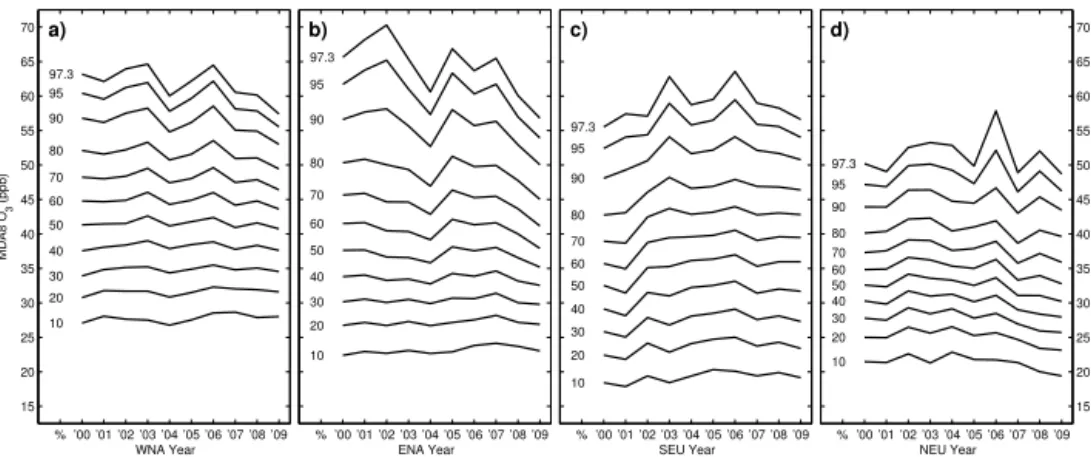
We seek a percentile that represents the cleanest air possible over the summer season (even if it is never realized during the summer), and one that does not change across years. We use MDA8 rather than 24 h average data to prevent night-time values from determining the baseline. We calculate per-centiles for each cell on an annual basis and then derive re-gional area-weighted averages of the percentiles. The result-ing percentiles by region (Fig. 2) show that the year-to-year variability is small below the 40th percentile, but the largest pollution years are evident at and above the 50th percentile. Thus, we select the 30th percentile as each grid cell’s base-line level, which corresponds roughly to the lower levels of spring–fall days. One might argue choosing, for example, the 10th percentile of JJA to estimate summertime enhancement; however, this assumes JJA in all models is the peak of the an-nual cycle and still sees clean air. We define O3enhancement
(EX, unit=ppb) here as the difference between the 30th
per-centile and any larger value, where subscripts will describe the reference value.
To estimate the summertime O3enhancement from local
to continental-scale pollution, we assume that the 92 days of JJA are the highest O3values of the year, pick their median
value (87th percentile), and subtract from it the spring–fall baseline (30th percentile). Maps of the summer enhancement EJJA (i.e., 87th minus 30th percentile) in NA and EU in
ob-servations and models are shown in Fig. 3. While O3levels
for the 87th, 30th, and other percentiles vary considerably from cell to cell (see S2014), the maps of observedEJJAshow
mostly large-scale structures.
Many models (A, B, D, E, F, H, I) have similar patterns of EJJA over NA, with large enhancements (30 to 50 ppb) from
the Mississippi through the Ohio River valley to the north-east, whereas the observations show such a pattern but with smaller enhancements (25 to 30 ppb). Model A greatly over-estimatesEJJA in the most polluted areas (e.g., California,
ar-% ’00 ’01 ’02 ’03 ’04 ’05 ’06 ’07 ’08 ’09 15
20 25 30 35 40 45 50 55 60 65 70
10 20 30 40 50 60 70 80 90 95 97.3
MDA8 O
3
(ppb)
WNA Year
a)
% ’00 ’01 ’02 ’03 ’04 ’05 ’06 ’07 ’08 ’09 10
20 30 40 50 60 70 80 90 95 97.3
ENA Year
b)
% ’00 ’01 ’02 ’03 ’04 ’05 ’06 ’07 ’08 ’09 10
20 30 40 50 60 70 80 90 95 97.3
SEU Year
c)
% ’00 ’01 ’02 ’03 ’04 ’05 ’06 ’07 ’08 ’09 15 20 25 30 35 40 45 50 55 60 65 70
10 20 30 40 50 60 70 80 90 95 97.3
NEU Year
d)
Figure 2.Values of MDA8 O3(ppb) for years 2000 to 2009 corresponding to the 10th, 20th,. . . , 90th, 95th, and 97.3 (i.e., AQX threshold)
percentiles in(a)WNA,(b)ENA,(c)SEU, and(d)NEU. The percentile for each line is shown at the beginning of the curves in each panel.
Figure 3.Summertime O3enhancementEJJAis the difference between the 87th and 30th percentile of the gridded surface MDA8 O3(ppb)
over (left two columns) NA and (right two columns) EU for the observations (O), ACCMIP models (A–H), and UCI CTM (I). The values of model I are scaled by 0.5 so the same color scale can be used.
eas near the Gulf of Mexico. The extremely large bias near the Gulf of Mexico is unique to model A, presumably
result-ing from natural JJA emission sources such as lightresult-ing NOx,
0 10 20 30 40 50 60 70 80 90 100
Percentage of events in episodes with areas >
S
a)
1 10 100 1,000 10,000
15 20 25 30 35 40 45 50 55
NA AQX Episode Size S (10 km - days)4 2
Enhancement (E
S
, ppb above 30
th percentile) c)
0 10 20 30 40 50 60 70 80 90 100
b)
1 10 100 1,000 10,000
15 20 25 30 35 40 45 50 55
4 2
d)
O (415 / 444) A (128 / 173) B (229 / 198) C (1426/2106) D (461 / 656) E (290 / 290) F (522 / 616) G (243 / 498) H (774 / 606) I (463 / 535)
EU AQX Episode Size S (10 km - days)
Figure 4. (a–b)Complementary cumulative distribution (CCD) of the percentage of total areal extent of all individual AQX events
(100-per-decade case) as a function of AQX episode size (S, 104km2days) for the observations (O), ACCMIP models (A–H), and UCI CTM (I) in(a)NA and (b) EU. Dashed vertical lines show the graphical representations of CCD100and CCD1000. Mean episode size (S) for each
data set and domain is given in the legend as (NA/EU).(c–d)Density scatterplot of the observations enhancement of AQX episodesESvs.
their sizeS(ESbinned at 2.5 ppb increments from < 15 ppb to > 55 ppb,Sbinned at each log decade) in (c) NA and (d) EU. The gray scale
represents the relative percentage of AQX episodes in each (x,y)=(S,ES) bin and includes percent ranges of≤5 % (white), 5–10, 10–15, and > 15 % (darkest gray) where the size bins (i.e., columns) are normalized to sum to 100 %. The overlain curves show the observation’s and each model’s area-weighted mean enhancementESfor each size bin. The values ofESin each size bin for models A and I have been
scaled by 0.5 since they are largely outside the range of the others.
large anthropogenic sources. Two models (C, G) are unusu-ally uniform across NA (except California). Surprisingly, this sorting of the models does not hold for EU. For example, there must be some clue as to why model B greatly overesti-matesEJJAover NA but underestimates it over EU. Such
be-havior from model C (uniformEJJA) may be expected since
the tropospheric VOC chemistry is highly simplified. The uniform pattern ofEJJAis also somewhat evident in EU for
model E, which has even simpler VOC chemistry compared to C, although this may be due to biases in the representation of physical climate rather than chemistry.
TheEJJAdiagnostic provides an excellent geographically
resolved test for CCM development. It also provides a useful measure of O3regional pollution changes in a future climate
with shifting O3baselines due to hemispheric-scale changes
in methane, water vapor, temperature, and stratospheric in-flux. Over each of our four regions, we calculate the aver-age summertime enhancementEJJA (see Tables 3 and S3 in
the Supplement), expecting to find the values and model–
measurement differences similar to those found in the sea-sonal amplitudeM. Indeed, this is true, albeitEJJA is
gen-erally smaller thanM. In addition, the spatial pattern of the values and model–measurement differences are also consis-tent betweenEJJAandM(not shown).
3.5 AQX episode size
For NA observations, the fraction of AQX area-weighted events that occur in episodes with S> 100×104km2 days (CCD100) is 79 %; and those with S> 1000×104km2
days (CCD1000) is 38 %. For EU observations, most AQX
events also occur in large episodes: CCD100=80 % and
CCD1000=35 %. Model C is aberrant in having extremely
large episodes (e.g., NA CCD100=93 %), which fall mostly
in the spring rather than summer months (see Fig. 1m–p). This may result from the model’s simplified chemistry or unrealistic widespread stratospheric intrusion of O3. In any
case, this model’s summertime high ozone events are ob-scured. Model A, with much more complex chemistry, how-ever, shows significantly smaller episodes. For CCD100, the
other models (B, D–I) are close to the observed: 73–85 % for NA and 71–85 % for EU. For CCD1000, however, this model
spread diverges substantially: 13–69 % for NA and 15–70 % for EU. In general, models A, B, E, and G do not produce the larger episodes and thus their physical climate may lack the synoptically correlated persistent stagnation episodes. The UCI CTM, using observed meteorology, captures the shape of the observed CCDs extremely well compared to the free-running climate of the ACCMIP models.
Integrating over all episodes, we calculate the weighted geometric mean size (S) (see S2014). Observations have mean episode sizes (S) of 415 (104 km2 days) and 444 in NA and EU, respectively. Models C, D, F, H, and I are bi-ased high in (S), while models A, B, E, and G are bibi-ased low for both NA and EU (Fig. 4a–b, Tables 3 and S4 in the Supplement).
3.6 Non-stationarity and possible trends
One problem with diagnosing decadal AQX size statistics is that they can be biased when more AQX events occur at one end of the decade due to a trend in O3 precursor
emis-sions. A greater density of events in one summer generally means larger episodes. A linear fit of annually derived O3
percentiles calculated over years 2000–2008 (2009 was ex-cluded due to lack of NOx and VOC emission data, see
be-low) for each of the four regions (Fig. S5 in the Supple-ment) shows clearly decreasing surface O3abundances at the
higher percentiles (see also Fig. 2), presumably through re-ductions in NOx and VOC emissions (Hudman et al., 2009;
Xing et al., 2014). To test if these trends are emission-driven or artifacts of the meteorological time slice, we analyze the UCI CTM results (dashed lines, Fig. S5 in the Supplement), which are forced by observed meteorology but have constant anthropogenic pollution emissions over the time period. We also obtain total NOx and VOC emissions from version 4.2
of the Emission Database for Global Atmospheric Research (EDGAR, EC-JRC/PBL, 2009) for years 2000–2008 (2009 was unavailable at time of publication) and calculate their trends over the period. Over WNA and ENA, meteorology seems to be driving the small positive trends at lower O3
per-centiles (where UCI and observed trends roughly agree), but
above the 60th percentile (where UCI and observed trends diverge) emissions reductions are the most likely cause. In SEU and NEU the trends are less conclusive for either me-teorology or emission based, but most EU NOx reductions
occurred prior to 2000 (Xing et al., 2015). Koumoutsaris and Bey (2012) compare GEOS-Chem hindcasts with NA and EU trends at a limited number of stations from CASTNet and EMEP (∼40 in each domain) and find similar trends. They also attribute the negative trends at high percentiles to reduced precursor emissions; however, they attribute the pos-itive trends at low percentiles to changing background O3as
opposed to changing meteorology posited here.
In an effort to correct the AQX decadal statistics for changes in O3 precursors, we searched for correlations on
a cell-by-cell basis between high-percentile MDA8 O3 vs.
NOxemissions on an annual basis for years 2000–2008. No
simple linear relation emerged, and we could find no satis-factory way to “correct” the observations for this regionally varying, monotonic but nonlinear, decline in NOxand VOC
emissions that did not corrupt the data. The post-CMIP5 plans for the Chemistry-Climate Model Initiative (CCMI) include hindcast simulations with time-dependent emissions that will allow for the simulation of the observed O3
non-stationarity.
One option for analyzing extremes in a non-stationary decadal data set is to define AQX events annually on a 10-per-year basis. This approach greatly dampens the observed episode mean size and across-year standard deviation from 415±307 (100 per decade) to 249±67 (10 per year) in NA and from 444±720 to 355±48 in EU. Moreover, it gives a false positive impression of the severity of air pollution in extreme years. Thus, we maintain our primary analysis with AQX defined as 100-per-decade. In parallel with Fig. 4a–b, we show the CCDs using a 10-per-year basis for AQX in Fig. S6a–b in the Supplement.
3.7 Severity of pollution in largest episodes
As a measure of O3produced during AQX events/episodes,
we map out the enhancement at the AQX threshold level EAQX (∼97.3 percentile) as shown in Fig. S7 in the
Sup-plement (parallel to Fig. 3, also relative to the local 30th percentile). We also calculate the average AQX enhance-mentEAQX over our regions (Tables 3 and S4 in the
Sup-plement). For ENA, the ACCMIP modeled range ofEAQXis
29–52 ppb, spanning the observed of 35 ppb (Table 3). This average result is encouraging for the ACCMIP models except that, as forEJJA(Fig. 3), the pattern match is not as good
(Ta-bles 3, S3 and S4 in the Supplement).
Of the 100 AQX events in each cell, many will lie above the local AQX threshold value. We expect that larger, longer-duration episodes accumulate more O3, and thus these
su-per episodes might have O3 enhancements (relative to the
(ppb) as the MDA8 value of that AQX event minus the local 30th percentile value. For each episode of sizeS, we calcu-late the area-weighted average enhancementES. Figure 4c–d
plot the observed density distribution of allES, quantized
ev-ery 2.5 ppb forESand every decade in 104km2days forS.
These plots show large variability in the observed ES
fre-quency (gray pixels) and yet a consistent picture of the mean enhancements as a function ofS(open circles). For episode sizes of 0.3 (i.e., 0.1 to 0.99), 3, and 30,ESis almost constant
(∼32 ppb for both NA and EU), but for sizes 300 and 3000 it increases almost linearly per decade. We calculate this slope 1ES as the average of the 30-to-300 increase (1 decade in
S) plus half of the 30-to-3000 increase (2 decades), getting values of 2.9 (NA) and 1.7 (EU) ppb increase per decade of episode size. Similar results are seen for the 10-per-year AQX definition (Fig. S6c–d in the Supplement), with1ES
of 2.7 (NA) and 3.3 (EU). The slope1ES is not simply an
expected result from our statistical sorting since in NA we find that compared to the observations, model C has slope that is a factor of about 4 smaller, while A has a slope nearly a factor of 4 larger, and F has a negative slope.
The models generally produce the shape ofES vs.S,
al-though most models (except A and I, see Fig. 4 caption) un-derestimate the enhancement for all sizes. The obvious dis-crepancies are for NA episodes, where many models predict that the largest enhancements occur in the smallest episodes (S=0.3). This anomaly does not occur for EU episodes. These small episodes are uncommon, representing only a small fraction of events (see Sect. 3.5), and we find them mostly along the coasts at the edge of the mask. We under-stand them to be the effect of very polluted air masses being advected to the neighboring ocean cells which are typically low-O3regions with very low 30th percentile baselines,
re-sulting in large enhancements from the highly polluted air. The observations are interpolated and not capable of follow-ing a pollution shift offshore. Thus the models are probably correct, but the method of masking and station interpolation makes this discrepancy a systematic feature. The lack of such a feature in EU can be understood by the lack of such sharp coastal gradients. Overall, most models agree with the obser-vations, showing that the super-episodes have the largest O3
enhancements.
4 Conclusions and discussion
Confidence in modeled projections of future air quality is based fundamentally on our ability to accurately simulate the present-day observed climatology of surface O3and
particu-late matter over NA and EU where dense, long-term, reliable measurements are available. In this work we evaluate the sur-face O3climatologies from eight global models (six CCMs,
one CTM, and one CGCM) that reported hourly surface O3
as part of the ACCMIP. In addition we test the UCI CTM simulation as an exact hindcast of the 2000–2009 decade
of observations used here. Our tests follow the unique ap-proach of S2014 in which over 4000 heterogeneously spaced air quality stations are used to calculate the hourly O3
aver-aged over 1◦×1◦grid cells that can then be compared un-ambiguously with the modeled grid. Diagnostics include the hourly diurnal cycle, monthly seasonal cycles, and sizes and intensity of air quality extreme episodes. For the most part, the models are biased high during all hours of the day, all months of the year, and in all regions.
Averaged over large regions, the ACCMIP models sim-ulate the shape of the observed summertime diurnal cycle well, with the hour of maximum within±1 h of observed (∼15:00 LT). The observed peak-to-peak amplitude (25 to 29 ppb over the more polluted regions) is not as well matched and typically underestimated by about 7 ppb. The UCI CTM hindcast, which performed well in the S2014 tests except for a uniform high bias, clearly fails these new diurnal tests and indicates model error in the morning boundary layer chem-istry. In general, the ACCMIP models simulate the observed regional annual cycle of monthly mean MDA8 O3. They
match the month of maximum to within±1 month of ob-served (mid-June), although two models are in error with al-most no annual cycle and no clear maximum. The other mod-els overestimate the peak-to-peak amplitude of the observed cycle by about 5 ppb (20 %) in the most polluted region (east-ern North America) while underestimating it by about 5 ppb in the other three regions. Model skill in matching the annual cycle of AQX events is fair but not good. This annual cycle has much larger interannual variability than that of MDA8 O3, and many models shift the month of maximum AQX
events to later in the summer than is observed.
Measures of the enhancement in surface O3driven by
pol-lution are derived from the statistics of the decade of daily gridded MDA8 values. For our measure of summertime en-hancement (87th minus 30th percentile), the models gener-ally replicate the observed spatial structures but overestimate the magnitude in the most polluted regions. Two models are surprisingly uniform across both continents and fail to high-light areas with the largest emissions of O3precursors.
Typ-ically, modeled high biases appear in the upper percentiles, not the 30th percentile, which appears to be a good measure of the baseline O3across the decade.
About 80 % of the AQX events in NA and EU occur in large, connected, multi-day episodes consisting of 100 grid cells or more. This result is closely matched by all but two models, with C producing much larger episodes and A much smaller ones. It remains unclear whether such errors result from chemical or physical processes. The observations show that super-sized episodes of 100 cells or more have succes-sively greater O3levels as they become bigger, with the
100-times-larger episodes having 4–6 ppb greater O3. Most, but
4.1 What are the best air quality diagnostics for model development?
For testing and identifying the model strengths and weak-nesses and improving simulations of air quality, modelers save a large number of diagnostics during the model devel-opment process. This typical model develdevel-opment process is far less limiting than the experiment analyzed here, which is based on the voluntary contributions of many models and many terabytes of diagnostics imposed in the ACCMIP. We would still recommend saving the diagnostic of hourly sur-face O3 over a decade or more of simulation from which
all of the primary diagnostics here can be readily derived and compared with the observations. To segue from the sur-face O3over NA and EU to the sondes and remote sites, a
monthly averaged 3-D O3 would probably suffice. Hourly
data observed at coastal or mountain sites likely include a di-urnal meteorology that is not represented in the global mod-els, even at a resolution of 0.5◦×0.5◦. Furthermore, the 24 h and MDA8 averages show different biases and should not be treated as the same diagnostic. There may be inventive ways to avoid the massive hourly data sets by storing the diurnal cycle as a monthly mean and calculating MDA8 inline or just storing the maximum daily O3value, which would then
re-quire similar analysis of the observations.
The open questions are what model simulations are prac-tical and which would be most useful to identify model er-rors. The ACCMIP simulations forced by a decade of 2000s climate-model sea surface temperatures are useful in com-paring decadal statistics, but the UCI CTM hindcast pro-vides unique tests on the ability to simulate specific events and years. Even if the observed sea surface temperatures were used, the synoptic extreme events would not likely co-incide with the observed, so a hindcast meteorology based on reanalysis for forecast fields provides an important test of the model.
The surface O3data here are based on an interpolation
al-gorithm that was optimized for the 50–100 km scale aver-ages. Thus, the supplied grid-cell averaged data could be re-generated at 0.5◦resolution, but if one wants 10 km cell av-erages for regional models then the parameters in the current algorithm would need to be revised and re-optimized. The surface O3data set will be expanded to include more than 2
decades (1993–2015) and thus longer simulations would be desirable to investigate interannual variability.
4.2 What are the most important tests for these chemistry–climate models, assuming that hindcasts and detailed emission data are not being used? Another major question is what emissions to use. With AC-CMIP the choice of a single year of representative emissions for the decade was the optimal choice. The downward trend-ing emissions in NA and EU over the 2000–2009 decade, however, created a non-stationary data set. Going to a longer
data set, 1993–2015, will make the comparison between models and measurements more awkward. Model develop-ers will need to take some account of this non-stationarity, possibly as a sensitivity study using two different emissions sets representative of the early and late periods of observa-tions, when not tracking emission changes each year.
An emissions problem not resolved here is whether the modeled diurnal cycle over heavily polluted regions in sum-mer would be affected by imposing a more accurate diurnal and weekly cycle in emissions. This is probably beyond what can be imposed in a model intercomparison project such as the ACCMIP but should be part of the individual model de-velopment as a sensitivity assessment.
The four-region decadal average statistics here provide a fairly broad view of the models’ ability to predict the buildup of O3and extreme events in polluted regions. Clear examples
of model error are identified. The general agreement of the diurnal cycle between models and measurements still needs to be tested with diurnal emissions. Going beyond the mean regional cycles, the ability to test models at the grid-cell level provides clear geographic coverage, identifying patterns of the discrepancy that are sometimes disturbing, as shown in Fig. 3, but not developed further in this paper. The next study of the CMIP-generated surface O3needs to evaluate this.
4.3 What tests provide the best confidence in model prediction of future air quality?
Accurate projections of future air quality rely on our ability to predict the changes in both baseline level and pollution buildup in response to both specified future climatic con-ditions and a change in local-to-global emissions. Both the baseline and the amount of O3produced from pollution are
likely to change and need to be assessed separately. For that purpose, we find that the maps of summertime (87th per-centile) and baseline (30th perper-centile) and their difference are one of the more important tests of a model’s simulation of the present day. The annual cycle of monthly means is also in some way a measure of the summertime enhance-ment but not as useful as the percentiles. One key measure of future change would be in the size and intensity of ex-treme episodes. The intensity needs to be assessed relative to the baseline, but the size of the episodes clearly relates to their intensity and would be independent of shifts in base-line. Thus the AQX statistics based on the daily MDA8 val-ues here are an important model test.
Acknowledgements. Research at UCI was supported by NASA grants NNX09AJ47G, NNX13AL12G, NNX15AE35G, and DOE award DE-SC0007021. J. L. Schnell was supported by the National Science Foundation’s Graduate Research Fellowship Program (DGE-1321846). The work of D. Bergmann and P. Cameron-Smith was funded by the US Dept. of Energy (BER), performed under the auspices of LLNL under contract DE-AC52-07NA27344, and used the supercomputing resources of NERSC under contract no. DE-AC02-05CH11231. G. Zeng acknowledges the use of New Zealand’s national HPC facilities that are provided by the NZ eScience Infrastructure and funded jointly by NeSI’s collaborator institutions and through the Ministry of Business, Innovation & Employment’s Research Infrastructure Programme. The simulations with MIROC-CHEM was supported by the Global Environment Research Fund (S-7) by the Ministry of the Environment Japan and completed with the supercomputer (NEC SX-8R) at the National Institute for Environmental Studies (NIES). We are grateful to the US Environmental Protection Agency’s (EPA) Air Quality System (AQS) and Clean Air Status and Trends Network (CASTNet), Environment Canada’s National Air Pollu-tion Surveillance Program (NAPS), the European Monitoring and Evaluation Programme (EMEP), and the European Environment Agency’s (EEA) air quality database (AirBase) for providing the observational data sets used in this study. We are also grateful to the British Atmospheric Data Centre (BADC), which is part of the NERC National Centre for Atmospheric Science (NCAS), for collecting and archiving the ACCMIP data.
Edited by: L. Ganzeveld
References
Barnes, E. A. and Fiore, A. M.: Surface ozone variability and the jet position: Implications for projecting future air quality, Geophys. Res. Lett., 40, 2839–2844, doi:10.1002/grl.50411, 2013. Büeker, P., Morrissey, T., Briolat, A., Falk, R., Simpson, D.,
Tuovi-nen, J.-P., Alonso, R., Barth, S., Baumgarten, M., Grulke, N., Karlsson, P. E., King, J., Lagergren, F., Matyssek, R., Nunn, A., Ogaya, R., Peñuelas, J., Rhea, L., Schaub, M., Uddling, J., Werner, W., and Emberson, L. D.: DO3SE modelling of soil
moisture to determine ozone flux to forest trees, Atmos. Chem. Phys., 12, 5537–5562, doi:10.5194/acp-12-5537-2012, 2012. Cameron-Smith, P., Lamarque, J. F., Connell, P., Chuang, C., and
Vitt, F.: Toward an Earth system model: atmospheric chemistry, coupling, and petascale computing, J. Phys.-Conf. Ser., 46, 343– 350, doi:10.1088/1742-6596/46/1/048, 2006.
Doherty, R. M., Wild, O., Shindell, D. T., Zeng, G., MacKenzie, I. A., Collins, W. J., Fiore, A. M., Stevenson, D. S., Dentener, F. J., Schultz, M. G., Hess, P., Derwent, R. G., and Keating, T. J.: Impacts of climate change on surface ozone and intercontinental ozone pollution: A multi-model study, J. Geophys. Res.-Atmos, 118, 3744–3763, doi:10.1002/jgrd.50266, 2013.
Donner, L. J., Wyman, B. L., Hemler, R. S., Horowitz, L. W., Ming, Y., Zhao, M., Golaz, J.-C., Ginoux, P., Lin, S. J., Schwarzkopf, M. D., Austin, J., Alaka, G., Cooke, W. F., Delworth, T. L., Freidenreich, S. M., Gordon, C. T., Griffies, S. M., Held, I. M., Hurlin, W. J., Klein, S. A., Knutson, T. R., Langenhorst, A. R., Lee, H.-C., Lin, Y., Magi, B. I., Malyshev, S. L., Milly, P. C. D.,
Naik, V., Nath, M. J., Pincus, R., Ploshay, J. J., Ramaswamy, V., Seman, C. J., Shevliakova, E., Sirutis, J. J., Stern, W. F., Stouffer, R. J., Wilson, R. J., Winton, M., Wittenberg, A. T., and Zeng, F.: The Dynamical Core, Physical Parameterizations, and Basic Simulation Characteristics of the Atmospheric Component AM3 of the GFDL Global Coupled Model CM3, J. Climate, 24, 3484– 3519, doi:10.1175/2011jcli3955.1, 2011.
European Commission, Joint Research Centre (JRC)/Netherlands Environmental Assessment Agency (PBL), EC-JRC/PBL, Emis-sion Database for Global Atmospheric Research (EDGAR), re-lease version 4.0., http://edgar.jrc.ec.europa.eu (last access: 23 August 2014), 2009.
Fiore, A. M., Dentener, F. J., Wild, O., Cuvelier, C., Schultz, M. G., Hess, P., Textor, C., Schulz, M., Doherty, R. M., Horowitz, L. W., MacKenzie, I. A., Sanderson, M. G., Shindell, D. T., Stevenson, D. S., Szopa, S., Van Dingenen, R., Zeng, G., Ather-ton, C., Bergmann, D., Bey, I., Carmichael, G., Collins, W. J., Duncan, B. N., Faluvegi, G., Folberth, G., Gauss, M., Gong, S., Hauglustaine, D., Holloway, T., Isaksen, I. S. A., Jacob, D. J., Jonson, J. E., Kaminski, J. W., Keating, T. J., Lupu, A., Marmer, E., Montanaro, V., Park, R. J., Pitari, G., Pringle, K. J., Pyle, J. A., Schroeder, S., Vivanco, M. G., Wind, P., Wojcik, G., Wu, S., and Zuber, A.: Multimodel estimates of intercontinen-tal source-receptor relationships for ozone pollution, J. Geophys. Res.-Atmos, 114, D04301, doi:10.1029/2008jd010816, 2009. Ganzeveld, L., Bouwman, L., Stehfest, E., van Vuuren, D. P.,
Eick-hout, B., and Lelieveld, J.: Impact of future land use and land cover changes on atmospheric chemistry-climate interactions, J. Geophys. Res., 115, D23301, doi:10.1029/2010JD014041, 2010. Hjellbrekke, A.-G., Solberg, S., and Fjæraa, A. M.: Ozone mea-surements 2011, EMEP/CCC-Report 3/2013, 0-7726, Tech. Rep., Norwegian Institute for Air Research, Norway, avail-able at: http://www.nilu.no/projects/CCC/reports/cccr3-2013. pdf (last access: 25 July 2013), 2013.
Holmes, C. D., Prather, M. J., Sovde, O. A., and Myhre, G.: Fu-ture methane, hydroxyl, and their uncertainties: key climate and emission parameters for future predictions, Atmos. Chem. Phys., 13, 285–302, doi:10.5194/acp-13-285-2013, 2013.
Horton, D. E., Skinner, C. B., Singh, D., and Diffenbaugh, N. S.: Occurrence and persistence of future atmospheric
stagnation events, Nature Clim. Change, 4, 698–703,
doi:10.1038/nclimate2272, 2014.
HTAP: Hemispheric Transport Of Air Pollution 2010, Part A: Ozone And Particulate Matter, United Nations, Geneva, Switzer-land, 2010.
Hudman, R. C., Murray, L. T., Jacob, D. J., Turquety, S., Wu, S., Millet, D. B., Avery, M., Goldstein, A. H., and Hol-loway, J.: North American influence on tropospheric ozone and the effects of recent emission reductions: Constraints from ICARTT observations, J. Geophys. Res.-Atmos, 114, D07302, doi:10.1029/2008jd010126, 2009.
Josse, B., Simon, P., and Peuch, V. H.: Radon global simulations with the multiscale chemistry and transport model MOCAGE, Tellus B, 56, 339–356, doi:10.1111/j.1600-0889.2004.00112.x, 2004.
Pro-jections and Predictability, in Climate Change 2013: The Phys-ical Science Basis, chapter 11, IPCC WGI Contribution to the Fifth Assessment Report, 2013.
Koch, D., Schmidt, G. A., and Field, C. V.: Sulfur, sea salt, and radionuclide aerosols in GISS ModelE, J. Geophys. Res.-Atmos, 111, D06206, doi:10.1029/2004jd005550, 2006.
Koumoutsaris, S. and Bey, I.: Can a global model reproduce ob-served trends in summertime surface ozone levels?, Atmos. Chem. Phys., 12, 6983–6998, doi:10.5194/acp-12-6983-2012, 2012.
Lamarque, J. F., Shindell, D. T., Josse, B., Young, P. J., Cionni, I., Eyring, V., Bergmann, D., Cameron-Smith, P., Collins, W. J., Do-herty, R., Dalsoren, S., Faluvegi, G., Folberth, G., Ghan, S. J., Horowitz, L. W., Lee, Y. H., MacKenzie, I. A., Nagashima, T., Naik, V., Plummer, D., Righi, M., Rumbold, S. T., Schulz, M., Skeie, R. B., Stevenson, D. S., Strode, S., Sudo, K., Szopa, S., Voulgarakis, A., and Zeng, G.: The Atmospheric Chemistry and Climate Model Intercomparison Project (ACCMIP): overview and description of models, simulations and climate diagnostics, Geosci. Model Dev., 6, 179–206, doi:10.5194/gmd-6-179-2013, 2013.
Lin, J. T., Youn, D., Liang, X. Z., and Wuebbles, D. J.: Global model simulation of summertime US ozone diurnal cycle and its sensi-tivity to PBL mixing, spatial resolution, and emissions, Atmos. Environ., 42, 8470–8483, doi:10.1016/j.atmosenv.2008.08.012, 2008.
Logan, J. A.: Ozone in rural-areas of the united-states, J. Geophys. Res.-Atmos, 94, 8511–8532, doi:10.1029/JD094iD06p08511, 1989.
Menut, L., Bessagnet, B., Colette, A., and Khvorostiyanov, D.: On the impact of the vertical resolution on
chemistry-transport modelling, Atmos. Environ., 67, 370–384,
doi:10.1016/j.atmosenv.2012.11.026, 2013.
Mickley, L., Jacob, D., Field, B., and Rind, D.: Effects of future climate change on regional air pollution episodes in the United States, Geophys. Res. Lett., 31, L24103, doi:10.1029/2004GL021216, 2004.
Naik, V., Horowitz, L. W., Fiore, A. M., Ginoux, P., Mao, J., Aghedo, A. M., and Levy II, H.: Impact of preindustrial to present-day changes in short-lived pollutant emissions on at-mospheric composition and climate forcing, J. Geophys. Res.-Atmos., 118, 8086–8110, doi:10.1002/jgrd.50608, 2013. National Research Council (US): Committee on the Significance of
International Transport of Air Pollutants. Global Sources of Lo-cal Pollution: An Assessment of Long-Range Transport of Key Air Pollutants to and from the United States, National Academies Press, Washington DC, 248 pp., 2009.
Oman, L. D., Ziemke, J. R., Douglass, A. R., Waugh, D. W., Lang, C., Rodriguez, J. M., and Nielsen, J. E.: The response of tropical tropospheric ozone to ENSO, Geophys. Res. Lett., 38, L13706, doi:10.1029/2011gl047865, 2011.
Prather, M., Gauss, M., Berntsen, T., Isaksen, I., Sundet, J., Bey, I., Brasseur, G., Dentener, F., Derwent, R., Stevenson, D., Gren-fell, L., Hauglustaine, D., Horowitz, L., Jacob, D., Mickley, L., Lawrence, M., von Kuhlmann, R., Muller, J. F., Pitari, G., Rogers, H., Johnson, M., Pyle, J., Law, K., van Weele, M., and Wild, O.: Fresh air in the 21st century?, Geophys. Res. Lett., 30, 1100, doi:10.1029/2002gl016285, 2003.
Reidmiller, D. R., Fiore, A. M., Jaffe, D. A., Bergmann, D., Cu-velier, C., Dentener, F. J., Duncan, B. N., Folberth, G., Gauss, M., Gong, S., Hess, P., Jonson, J. E., Keating, T., Lupu, A., Marmer, E., Park, R., Schultz, M. G., Shindell, D. T., Szopa, S., Vivanco, M. G., Wild, O., and Zuber, A.: The influence of foreign vs. North American emissions on surface ozone in the US, At-mos. Chem. Phys., 9, 5027–5042, doi:10.5194/acp-9-5027-2009, 2009.
Schnell, J. L., Holmes, C. D., Jangam, A., and Prather, M. J.: Skill in forecasting extreme ozone pollution episodes with a global atmospheric chemistry model, Atmos. Chem. Phys., 14, 7721– 7739, doi:10.5194/acp-14-7721-2014, 2014.
Scinocca, J. F., McFarlane, N. A., Lazare, M., Li, J., and Plummer, D.: Technical Note: The CCCma third generation AGCM and its extension into the middle atmosphere, Atmos. Chem. Phys., 8, 7055–7074, doi:10.5194/acp-8-7055-2008, 2008.
Seinfeld, J. H., Atkinson, R., Berglund R. L., Chameides, W. L., Elston, J. C., Fehsenfeld, F., Finlayson-Pitts, B. J., Harriss, R. C., Kolb, C. E., Lioy, P. J., Logan, J. A., Prather, M. J., Russell, A., and Steigerwald, B.: Rethinking the ozone problem in urban and regional air pollution, National Academy Press, Washington, DC, 524 pp., 1991.
Shindell, D. T., Pechony, O., Voulgarakis, A., Faluvegi, G., Nazarenko, L., Lamarque, J. F., Bowman, K., Milly, G., Kovari, B., Ruedy, R., and Schmidt, G. A.: Interactive ozone and methane chemistry in GISS-E2 historical and future climate simulations, Atmos. Chem. Phys., 13, 2653-2689, doi:10.5194/acp-13-2653-2013, 2013.
Tang, Q. and Prather, M. J.: Correlating tropospheric column ozone with tropopause folds: the Aura-OMI satellite data, Atmos. Chem. Phys., 10, 9681–9688, doi:10.5194/acp-10-9681-2010, 2010.
Taylor, K. E.: Summarizing multiple aspects of model performance in a single diagram, J. Geophys. Res.-Atmos., 106, 7183–7192, doi:10.1029/2000jd900719, 2001.
Teyssèdre, H., Michou, M., Clark, H. L., Josse, B., Karcher, F., Olivié, D., Peuch, V.-H., Saint-Martin, D., Cariolle, D., Attié, J.-L., Nédélec, P., Ricaud, P., Thouret, V., van der A, R. J., Volz-Thomas, A., and Chéroux, F.: A new tropospheric and strato-spheric Chemistry and Transport Model MOCAGE-Climat for multi-year studies: evaluation of the present-day climatology and sensitivity to surface processes, Atmos. Chem. Phys., 7, 5815– 5860, doi:10.5194/acp-7-5815-2007, 2007.
Val Martin, M., Heald, C. L., and Arnold, S. R.: Coupling dry depo-sition to vegetation phenology in the Community Earth System Model: Implications for the simulation of surface O3, Geophys.
Res. Lett., 41, 2988–2996, doi:10.1002/2014GL059651, 2014. Wackernagel, H.: Multivariate Geostatistics: An introduction with
applications, 3rd ed., Springer, Berlin, 387 pp., 2003.
Watanabe, S., Hajima, T., Sudo, K., Nagashima, T., Takemura, T., Okajima, H., Nozawa, T., Kawase, H., Abe, M., Yokohata, T., Ise, T., Sato, H., Kato, E., Takata, K., Emori, S., and Kawamiya, M.: MIROC-ESM 2010: model description and basic results of CMIP5-20c3m experiments, Geosci. Model Dev., 4, 845–872, doi:10.5194/gmd-4-845-2011, 2011.
fu-ture changes in surface ozone: a parameterized approach, At-mos. Chem. Phys., 12, 2037–2054, doi:10.5194/acp-12-2037-2012, 2012.
Xing, J., Mathur, R., Pleim, J., Hogrefe, C., Gan, C.-M., Wong, D. C., Wei, C., Gilliam, R., and Pouliot, G.: Observations and mod-eling of air quality trends over 1990-2010 across the Northern Hemisphere: China, the United States and Europe, Atmos. Chem. Phys., 15, 2723–2747, doi:10.5194/acp-15-2723-2015, 2015. Young, P. J., Archibald, A. T., Bowman, K. W., Lamarque, J. F.,
Naik, V., Stevenson, D. S., Tilmes, S., Voulgarakis, A., Wild, O., Bergmann, D., Cameron-Smith, P., Cionni, I., Collins, W. J., Dal-soren, S. B., Doherty, R. M., Eyring, V., Faluvegi, G., Horowitz, L. W., Josse, B., Lee, Y. H., MacKenzie, I. A., Nagashima, T., Plummer, D. A., Righi, M., Rumbold, S. T., Skeie, R. B., Shin-dell, D. T., Strode, S. A., Sudo, K., Szopa, S., and Zeng, G.: Pre-industrial to end 21st century projections of tropospheric ozone from the Atmospheric Chemistry and Climate Model Intercom-parison Project (ACCMIP), Atmos. Chem. Phys., 13, 2063– 2090, doi:10.5194/acp-13-2063-2013, 2013.
Zeng, G., Pyle, J. A., and Young, P. J.: Impact of climate change on tropospheric ozone and its global budgets, Atmos. Chem. Phys., 8, 369–387, doi:10.5194/acp-8-369-2008, 2008.