Nat. Hazards Earth Syst. Sci., 8, 775–777, 2008 www.nat-hazards-earth-syst-sci.net/8/775/2008/ © Author(s) 2008. This work is distributed under the Creative Commons Attribution 3.0 License.
Natural Hazards
and Earth
System Sciences
Detection of ULF electromagnetic emissions as a precursor to an
earthquake in China with an improved polarization analysis
Y. Ida1, D. Yang2, Q. Li2, H. Sun3, and M. Hayakawa1
1Department of Electronic Engineering and Research Station on Seismo Electromagnetics,
The University of Electro-Communications, 1-5-1 Chofugaoka, Chofu, Tokyo, 182-8585, Japan
2Institute of Geophysics, China Earthquake Administration, Beijing 100081, China 3Kashi Observatory, Earthquake Administration of Xinjiang Uygur Autonomous Region,
Xinjiang 844000, China
Received: 16 May 2008 – Accepted: 1 July 2008 – Published: 30 July 2008
Abstract.An improved analysis of polarization (as the ratio of vertical magnetic field component to the horizontal one) has been developed, and applied to the approximately four years data (from 1 March 2003 to 31 December 2006) ob-served at Kashi station in China. It is concluded that the po-larization ratio has exhibited an apparent increase only just before the earthquake on 1 September 2003 (magnitude = 6.1 and epicentral distance of 116 km).
1 Introduction
There have been recently accumulated a lot of evidences on electromagnetic emissions in a wide frequency range associated with earthquakes (EQs) (e.g., Hayakawa and Molchanov, 2002; Molchanov and Hayakawa, 2008). The lowest frequency range, ULF (ultra low frequency, with fre-quency less than 10 Hz) is of practical importance in short-term EQ prediction, because they are able to propagate easily up to the Earth’s surface where a ULF sensor is installed.
The serious problem regarding these seismogenic ULF emissions is how to detect these weak signals. There have been developed different kinds of methods for the analysis; (1) polarization analysis by means of the ratio of vertical magnetic field component to the horizontal (Hayakawa et al., 1996), (2) fractal analysis (mono- and multi-) (Hayakawa et al., 1999; Gotoh et al., 2004; Smirnova et al., 2004; Ida and Hayakawa, 2006; Ida et al., 2005), (3) Principal component analysis (Gotoh et al., 2002) and singular value decomposi-tion (Hattori et al., 2006), and so on.
Correspondence to:M. Hayakawa [email protected]
In this paper we will use the polarization analysis as the simplest analysis method, but we have developed its im-proved one. This imim-proved polarization method is applied to the ULF data observed in China during four years. We try to find out any significant precursory effect for two EQs in China near the observing situation of Kashi in Fig. 1. Finally, the results obtained in this paper would be compared with earlier results for the 1993 Guam EQ (Hayakawa et al., 1996, 1999) and Kagoshima EQs in 1999 (Hattori et al., 2006).
2 ULF geomagnetic data and EQs
ULF geomagnetic data are obtained at an observatory named Kashi (geographic coordinates; 39.5◦
N, 76.0◦
E) as in Fig. 1. At this field site we observe three geomagnetic components (H:N Scomponent,D:EW component, andZ:vertical
com-ponent) by means of fluxgate sensors. The sampling fre-quency is 1 Hz. Nearly four years data are utilized for the analysis: 1 March 2003 through 31 December 2006.
There were observed two rather big EQs (with magnitude greater than 6.0) near the ULF station of Kashi; an EQ on 1 September 2006 and another EQ on 25 February 2005. The magnitude of the former one isM=6.1 and that of the latter one isM=6.0. The distance of the former EQ with respect to the observatory is about 116 km, while the epicenter distance for the next EQ is about∼300 km.
3 Polarization analysis
Polarization method as developed by Hayakawa et al. (1996) is based on the measurement of the ratio of spectral power of the vertical magnetic field (Z) to the horizontal magnetic
776 M. Hayakawa et al.: Seismo-ULF electromagnetic emissions
72˚ 74˚ 76˚ 78˚ 80˚ 38˚
40˚ 42˚
0 50 100
km
0 20 40 60 80 100
Depth
km
China
Kyrgyzstan
Tajikistan
Geographic latitude [deg]
Geographic longitude [deg]
Kashi
Geographic longitude [deg]Geographic latitude [deg]
60 70 80 90 100 110 120 130 140 20
30 40 50
Kashi
2003/09/01 M6.0
2005/02/14 M6.2
2005/02/25 M6.1
Fig. 1. The relative location of a ULF geomagnetic observatory, Kashi and two EQs (indicated by circles) occurred during the period of March 2003 to December 2006.
fields (H andD) (i.e.,Z/H orZ/D). This ratio is known to provide us with a lot of information whether the ob-served variation is of ionospheric orgin (or solar-terrestorial effect) or seismic-related. Generally speaking, the polariza-tion ratio becomes generally larger when we have seismo-genic emissions, while the geomagnetic variation is found to have smaller values (Hayakawa et al., 1996).
The time series ULF data are subject to the following sig-nal processing. The use of FFT enables us to change the time series information into the frequency domain. The window size used is 1024, and the window function is Hamming. The analysis window is shifted without any overlapping. Sec-ondly, the data at the frequency around 0.01 Hz (10 mHz) is picked up from the FFT result. This frequency is already known to represent seismogenic ULF emissions (Hayakawa et al., 2007), and this point was checked in this paper as well by changing the frequency in the analysis. The geomag-neticD component at∼0.01 Hz has a significant variation
at the terminator time (Zomer et al., 2008), while geomag-neticH andZcomponents at day exhibit significant annual variations. Additionally, daytime geomagnetic data are likely to include more artificial noise than at night. So that, the average of each geomagnetic component (H,D andZ) is computed by using the data from U.T.=18:00 to 21:00 (lo-cal nighttime) in order to reduce these effects. The values of
Z/HandZ/Dare computed as representing the daily data.
0.0 0.5 1.0 1.5 2.0 2.5 3.0 3.5 4.0
Z/H
0.0 0.5 1.0 1.5 2.0 2.5 3.0 3.5 4.0
Z/D
-450 -300 -150 0
Dst[nT]
January July January July January July January July
2003 2004 2005 2006
0 30
60Σ
Kp
Eq(2003/09/01)
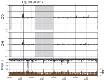
Fig. 2. Temporal polarization (Z/D, Z/H) results (before stan-dardization), Dst and6Kp indices. Eq is the EQ occurrence date.
4 Observational results on polarization
Figure 2 illustrates the temporal evolution of the polariza-tion analysis (Z/DandZ/H) during the whole period from March 2003 to December 2006. The shaded areas indicate the periods of no observation due to some problems of the ULF system. A vertical line indicates the day of occurrence of the nearby EQ on 1 September 2003. The upper part of the bottom panel refers to the geomagnetic activity expressed by Dst [nT], while the lower part indicates the6Kp index. It is seen from this figure that a certain enhancement is seen in theZ/D plot just before the EQ and also a less significant increase is seen in theZ/H plot. However, we can notice so many other peaks in both plots ofZ/D andH /D. So that, we cannot say anything about the correlation between the polarization and an EQ. The two plots ofZ/DandH /D
are seen to have no correlation with either Dst or6Kp. It is then likely that major causes for increasing the polarization during all the periods might be related to the different vari-ability in each geomagnetic field component. Because the average and standard deviation of each field is very different. So, we propose an improved polarization method in the following. Because of different behavior in each field com-ponent, we propose the standardization (normalization) of each geomagnetic field component as follows, which enables us to treat each field component equally. The standardized field component is defined by,
Ei=(Xi−µi)/σi
whereXi is the average value for one day mean for the i
component (i=H, DandZ),µiis the average of the
compo-nent i over the whole period, andσiis the standard deviation
of the same componentiover the whole period. An increase
M. Hayakawa et al.: Seismo-ULF electromagnetic emissions 777 in the polarization is resulted from not only an increase inZ,
but also from a decrease inH orD. So that, only when the standardized value ofH or D component is exceeding 0.1 (that is, any significant change is observed), we compute the polarization and the corresponding result is given in Fig. 3.
It is seen that Fig. 3 is completely different from the re-sult in Fig. 2. In this figure both values ofZ/D andZ/H
are found to exhibit a significant increase only before the EQ, and no any significant changes are observed during the whole period. The indices of Dst and6Kp did not show any changes before the EQ, which means that the increase in polarization before the EQ has nothing to do with the geo-magnetic activity, but it is closely associated the EQ.
As regards the second EQ on 25 February 2005, there seems to exhibit no any significant change. The epicentral distance for this EQ is about 300 km, which is too far to de-tect any seismogenic effects (Hayakawa et al., 2007).
5 Concluding remarks
An improved polarization method developed in this paper is applied to the ULF data at Kashi station in China. Three geo-magnetic field components behave in a different way, so that we have adopted general standardization (or normalization) by estimating the average and standard deviation during the whole period for each component. By using these standard-ized geomagnetic field quantities, it is found that the polar-ization as the ratio of vertical magnetic field component to that of horizontal magnetic field component (Z/H, Z/Dat a particular frequency of∼0.01 Hz (10mHz) exhibits a
sig-nificant increase only before the EQ on 1 September 2003 (magnitude=6.0 and epicentral distance=120 km). We com-ment on the lead time for this EQ; that is, during 1 August to the end of August, we notice the enhancement in the polar-ization, with the maximum polarization value a few days be-fore the EQ. This kind of ULF lead time seems to be consis-tent with earlier works by Hayakawa et al. (1996) and Hattori et al. (2006). No effect in ULF emissions is observed for the 2nd EQ on 25 February 2005, which can be easily understood in terms of a larger epicentral distance of ∼300 km, being
consistent with earlier statistics by Hayakawa et al. (2007).
Edited by: M. Contadakis
Reviewed by: two anonymous referees
References
Gotoh, K., Akinaga, Y., Hayakawa, M., and Hattori, K.: Princi-pal component analysis of ULF geomagnetic data for Izu islands earthquakes in July 2000, J. Atmos. Electr., 22, 1–12, 2002. Gotoh, K., Hayakawa, M., Smirnova, N. A., and Hattori, K.: Fractal
analysis of seismogenic ULF emissions, Phys. Chem. Earth, 29, 419–424, 2004.
Hattori, K., Serita, A., Yoshino, C., Hayakawa, M., and Isezaki, N.: Singular spectral analysis and principal component analysis for signal discrimination of ULF geomagnetic data associated with
-10 -5 0 5 10
Z/D
-450 -300 -150 0
Dst[nT]
January July January July January July January July
2003 2004 2005 2006
0 30 60ΣKp
Eq(2003/09/01)
-10 -5 0 5 10
Z/H
Fig. 3.Temporal evolution on the polarization (Z/D, Z/H) results after standardization, Dst and6Kp indices. Eq is the EQ occur-rence date.
2000 Izu Island earthquake swarm, Phys. Chem. Earth, 31, 281– 291, 2006.
Hayakawa, M., Kawate, R., Molchanov, O. A., and Yumoto, K.: Re-sults of ultra-low-frequency magnetic field measurements during the Guam earthquake of 8 August 1993, Geophys. Res. Lett., 23, 241–244, 1996.
Hayakawa, M., Itoh, T., and Smirnova, N.: Fractal analysis of ULF geomagnetic data associated with the Guam earthquake on 8 Au-gust 1993, Geophys. Res. Lett., 26(18), 2797–2800, 1999. Hayakawa, M. and Molchanov, O. A.: Seismo Electromagnetics:
Lithosphere – Atmosphere – Ionosphere Coupling, TERRAPUB, Tokyo, Japan, p. 477, 2002.
Hayakawa, M., Hattori, K., and Ohta, K.: Monitoring of ULF (ultra-low-frequency) geomagnetic variations associated with earth-quakes, Sensors, 7, 1108–1122, 2007.
Ida, Y., Hayakawa, M., Adalev, A., and Gotoh, K.: Multifractal analysis for the ULF geomagnetic data during the 1993 Guam earthquake, Nonlinear Proc. Geoph., 12, 157–162, 2005. Ida, Y. and Hayakawa, M.: Fractal analysis for the ULF data during
the 1993 Guam earthquake to study prefracture criticality, Non-linear Proc. Geoph., 13, 409–412, 2006.
Molchanov, O. A. and Hayakawa, M.: Seismo-Electromagnetics and Related Phenomena, History and latest results, TERRAPUB, Tokyo, Japan, p. 189, 2008.
Smirnova, N., Hayakawa, M., and Gotoh, K.: Precursory behav-ior of fractal characteristics of the ULF electromagnetic fields in seismic active zones before strong earthquakes, Phys. Chem. Earth, 29, 445–451, 2004.
Zomer, A., Price, C., Alperovich, C., Finkelstein, M., and Merzer, M.: ULF amplitude observations at the dawn/dusk terminators, J. Atmos. Electr., 28, 21–29, 2008.