Mixed layer variability and chlorophyll <i>a</i> biomass in the Bay of Bengal

(1)

BGD

10, 16405–16452, 2013

Mixed layer variability and chlorophylla

biomass

J. Narvekar and S. Prasanna Kumar

Title Page

Abstract Introduction

Conclusions References

Tables Figures

◭ ◮

Back Close

Full Screen / Esc

Printer-friendly Version

Interactive Discussion

Discussion

P

a

per

|

D

iscussion

P

a

per

|

Discussion

P

a

per

|

Discuss

ion

P

a

per

|

Biogeosciences Discuss., 10, 16405–16452, 2013 www.biogeosciences-discuss.net/10/16405/2013/ doi:10.5194/bgd-10-16405-2013

Open Access

Biogeosciences

Discussions

This discussion paper is/has been under review for the journal Biogeosciences (BG). Please refer to the corresponding final paper in BG if available.

Mixed layer variability and chlorophyll

a

biomass in the Bay of Bengal

J. Narvekar and S. Prasanna Kumar

CSIR-National Institute of Oceanography, Dona Paula, Goa 403 004, India

Received: 3 September 2013 – Accepted: 11 September 2013 – Published: 24 October 2013

Correspondence to: S. Prasanna Kumar (prasanna@nio.org)

(2)

BGD

10, 16405–16452, 2013

biomass

Title Page

Tables Figures

◭ ◮

Back Close

Full Screen / Esc

Discussion

P

a

per

|

D

iscussion

P

a

per

|

Discussion

P

a

per

|

Discuss

ion

P

a

per

|

Abstract

Mixed layer is the most variable and dynamically active part of the marine environ-ment that couples the underlying ocean to the atmosphere and plays an important role in determining the chlorophyll concentration. In this paper we examined the seasonal variability of the mixed layer depth in the Bay of Bengal, the factors responsible for it and 5

the coupling of mixed layer processes to the chlorophyll biomass using a suite of in situ as well as remote sensing data. The basin-wide mixed layer depth was the shallowest during spring intermonsoon, which was associated with strong themohaline stratifica-tion of the upper water column. The prevailing winds which were the weakest of all the seasons were unable to break the stratification leading to the observed shallow mixed 10

layer. Consistent with the warm oligotrophic upper ocean, the surface chlorophyll con-centrations were the least and the vertical profile of chlorophyll was characterized by a subsurface chlorophyll maximum. Similarly, during summer though the monsoon winds were the strongest they were unable to break the upper ocean haline-stratification in the northern Bay brought about by a combination of excess precipitation over evapo-15

ration and fresh water influx from rivers adjoining the Bay of Bengal. Consistent with this though the nitrate concentrations were high in the northern part of the Bay, the chlorophyll concentrations were low indicating the light limitation. In contrast, in the south, advection of high salinity waters from the Arabian Sea coupled with the west-ward propagating Rossby waves of annual periodicity were able to decrease stability 20

of the upper water column and the prevailing monsoon winds were able to initiate deep mixing leading to the observed deep mixed layer. The high chlorophyll concentration observed in the south resulted from the positive wind stress curl which pumped nutrient rich subsurface waters to the euphotic zone. The southward extension of the shallow mixed layer in fall intermonsoon resulted from the advection of low salinity waters from 25

(3)

BGD

10, 16405–16452, 2013

biomass

Title Page

Tables Figures

◭ ◮

Back Close

Full Screen / Esc

Discussion

P

a

per

|

D

iscussion

P

a

per

|

Discussion

P

a

per

|

Discuss

ion

P

a

per

|

mixed layer during winter resulted from a combination of reduced short wave radiation, increase in salinity and comparatively stronger winds. The mismatch between the low

nitrate and comparatively higher chlorophyll biomass during winter indicated the effi

-cacy of the limited nitrate data to adequately resolve the coupling between the mixed layer processes and the chlorophyll biomass.

5

1 Introduction

The upper ocean experiences large spatio-temporal variability compared to the rest of the ocean and hence it forms an important region for understanding both short-term and long-short-term changes including climate change. The intense mixing in the upper ocean by heat, momentum and freshwater flux results in the formation of a homoge-10

neous layer with nearly-uniform properties known as mixed layer. It is this layer that cou-ples the underlying ocean to the atmosphere through the transfer of mass and energy. The heat stored in the mixed layer regulates the air-sea exchange processes including convection and cyclone genesis. In addition, bulk of the oceanic biological productivity critically depends on the physical and chemical changes taking place within this layer. 15

Spatially the mixed layer thickness increases from few tens of meters at the equator to few hundreds of meter at the poles (Monterey and Levitus, 1997), while temporally it could vary from diurnal to inter-annual time scales (Weller and Farmer, 1992; Brainerd and Gregg, 1995; Kara et al., 2003). However, within a given geographical region, such as tropics, the structure and variability of mixed layer largely depends on the regional 20

oceanographic characteristics and atmospheric forcing.

The Bay of Bengal situated in the eastern part of the northern Indian Ocean is a tropical basin, which is landlocked in the north and is forced by semi-annually revers-ing monsoon wind system. The strongest winds occur durrevers-ing summer monsoon (June– September) when the southwesterly winds bring humid maritime air mass into the Bay 25

(4)

BGD

10, 16405–16452, 2013

biomass

Title Page

Tables Figures

◭ ◮

Back Close

Full Screen / Esc

Discussion

P

a

per

|

D

iscussion

P

a

per

|

Discussion

P

a

per

|

Discuss

ion

P

a

per

|

dry continental air mass to the Bay of Bengal. The unique feature of the Bay of

Ben-gal is the large seasonal freshwater influx from rivers (1.625×1012m3yr−1,

Subrama-nian, 1993) as well as excess precipitation over evaporation (∼2 m yr−1, Prasad, 1997),

which makes the waters of the upper layers less saline and highly stratified. This fresh water input leads to the formation of strong halocline within the upper isothermal layer 5

known as “barrier layer” (Lukas and Linderstrom, 1991; Sprintall and Tomczak, 1992). In the past several studies attempted to understand the mixed layer variability in the Indian Ocean including Bay of Bengal. There exist a few climatologies of the mixed layer depth for the tropical Indian Ocean (Colborn, 1975; Robinson et al., 1979; Levitus, 1982; Hastenrath and Greisher, 1989; Rao et al., 1989). Based on the time series data 10

collected during MONSOON-77 and MONEX-79, Gopalakrishna et al. (1988) studied the influence of wind on the variability of the mixed layer in the northern Indian Ocean

during different phases of summer monsoon. Using global ocean temperature

clima-tology, Rao and Sivakumar (2000) studied the near surface thermal structure and heat budget of the mixed layer of the tropical Indian Ocean including Bay of Bengal. Han 15

et al. (2001) showed that in the regions where precipitation exceeds evaporation the mixed layer was found to be thin because of decreased entrainment and increased barrier layer. While comparing the total kinetic energy available for mixing in the Ara-bian Sea and the Bay of Bengal, Shenoi et al. (2002) stated that the shallow mixed layer depth in the Bay of Bengal during the summer monsoon is primarily driven by 20

a combination of weaker winds and strong near-surface stratification. Subsequently, Vinaychandran et al. (2002) argued that strong stratification associated with the barrier layer curtails the vertical mixing leading to the formation of shallow mixed layers. In contrast, with help of one dimensional turbulent closure model Prasad (2004) studied the physical mechanism governing the seasonal evolution of mixed layer depth along 25

(5)

BGD

10, 16405–16452, 2013

biomass

Title Page

Tables Figures

◭ ◮

Back Close

Full Screen / Esc

Discussion

P

a

per

|

D

iscussion

P

a

per

|

Discussion

P

a

per

|

Discuss

ion

P

a

per

|

Narvekar and Prasanna Kumar (2006) examined the seasonal cycle of mixed layer in the central Bay of Bengal and its association to chlorophyll using more comprehensive data set including Argo data. Using global general circulation model De Boyer Mon-tegut et al. (2007) studied the mixed layer heat budget of the Bay of Bengal as a part of northern Indian Ocean and stated that the salinity stratification plays a clear role in 5

maintaining a high winter SST in the Bay of Bengal while presence of freshwater near the surface allows heat storage below the surface layer that can later be recovered by entrainment warming during winter cooling. More recently, Keerthi et al. (2012) studied the inter-annual variability of the mixed layer in the tropical Indian Ocean and its link to climate modes using eddy permitting numerical simulation and in situ hydrographic 10

data.

All of the above studies examined the variability of the mixed layer in the context of wind-mixing, net heat flux and fresh water flux. Most of them used monthly mean climatlogy of in situ data to address the mixed layer variability over Indian Ocean of which Bay of Bengal forms a part. The rest of the study used in situ data collected from 15

a limited spatial and temporal coverage in the Bay of Bengal during a particular cruise. Though the above studies yielded a fairly good understanding of the processes control-ling the mixed layer variability in the Bay of Bengal, there are several aspects which are yet to be addressed such as role of advection and remote forcing. More importantly,

we do not yet understand with sufficient details the role of mixed layer in regulating

20

the basin-wide variability in chlorophyll biomass and primary productivity. It is in this context that the present paper attempts to understand (1) processes controlling basin-wide variability of the mixed-layer and (2) coupling between mixed layer and chlorophyll biomass in the Bay of Bengal on a seasonal scale. In the present study using a more comprehensive quality-controlled hydrographic data and atmospheric data we explore 25

(6)

BGD

10, 16405–16452, 2013

biomass

Title Page

Tables Figures

◭ ◮

Back Close

Full Screen / Esc

Discussion

P

a

per

|

D

iscussion

P

a

per

|

Discussion

P

a

per

|

Discuss

ion

P

a

per

|

2 Data and methodology

In order to study the seasonal variability of mixed layer in the Bay of Bengal in response to the local and remote forcing and its coupling to basin-scale distribution of chlorophyll, a suite of both in-situ and remote sensing data pertaining to oceanographic and atmo-spheric parameters were used. The domain within which both the oceanographic and 5

meteorological data extracted were for the region equator to 25◦_{N latitude and 75}◦ _to

100◦_{E longitude.}

2.1 Hydrographic data

The hydrographic data pertaining to temperature and salinity was extracted from the following 3 sources:

10

1. The World Ocean Data base 2005 (WOD05) (Boyer et al., 2006) contained tem-perature and salinity data from Hydro-cast for the period 1919 to 2000 and con-ductivity temperature-depth (CTD) profiles for the period 1972 to 2003 (http: //www.nodc.noaa.gov/OC5/WOD05/pr_wod05.html).

2. Responsible National Oceanographic Data Center (RNODC) at National Institute 15

of Oceanography (CSIR-NIO), Goa which contained temperature and salinity data from Hydro-cast for the period 1972–1996 and CTD profiles for the period 1979– 2006. All the data were collected on board Indian research ships.

3. Argo data which contained the temperature and salinity profiles for the period 2002 to 2007 were extracted from http://www.usgodae.org/argo/argo.html. 20

In all 7197 profiles of temperature and salinity from Hydro-cast, 2714 profiles from CTD and 4569 profiles from Argo were extracted. These profiles were subjected to the following quality control procedures to obtain quality data for further analysis.

(7)

BGD

10, 16405–16452, 2013

biomass

Title Page

Tables Figures

◭ ◮

Back Close

Full Screen / Esc

Discussion

P

a

per

|

D

iscussion

P

a

per

|

Discussion

P

a

per

|

Discuss

ion

P

a

per

|

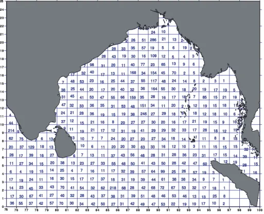
data were physically examined and duplicate profiles as well as those with obvious er-rors were excluded. After the quality control, the total number of Hydro-cast profiles was reduced to 5328 (882 RNODC & 4446 WOD05), CTD profiles to 2656 (1803 RNODC & 853 WOD05) and Argo profiles to 4203. From the quality checked data the spatial

dis-tribution of total number of temperature and salinity profiles available on a 1◦_{latitude by}

5

1◦_{longitude grids is presented in Fig. 1, while total number of profiles for each month is}

given in Table 1. From the quality-controlled temperature and salinity profiles, density

(sigma-t) was calculated (UNESCO, 1981) up to a depth of 500 m. This data was

fur-ther used to prepare monthly mean climatology of temperature, salinity and sigma-ton

a 1◦ _{latitude by 1}◦ _{longitude grids. These profiles were used to determine mixed layer}

10

depth (MLD).

In order to determine the mixed layer depth one could either specify a difference in

temperature or density (sigma-t) from the surface value (Wyrtki, 1964; Levitus, 1982;

Schneider and Muller, 1990) or specify a gradient in temperature or density (sigma-t)

(Bathen, 1972; Lukas and Lindstrom, 1991) depending upon the vertical structure of 15

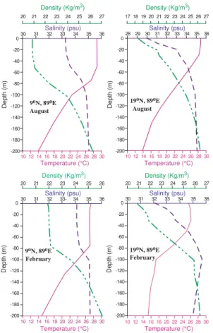
temperature, salinity and sigma-t of the region. An examination of the vertical profiles

of temperature, salinity and density (sigma-t) at two locations representing the northern

(19◦_{N, 89}◦_{E) and southern (9}◦_{N, 89}◦_{E) Bay of Bengal during February (winter) and}

August (summer) showed that in the southern part of the Bay of Bengal the isothermal, isohaline and isopycnal layers, in general, coincided in the upper ocean irrespective 20

of the season (Fig. 2 left panels). In the northern part of the Bay of Bengal there was practically no isohaline layer in the vertical profile of salinity and the salinity rapidly increased within the isothermal layer (Fig. 2 right panels). However, at times the salinity profile showed a thin isohaline layer in the upper water column (not shown). In view of the above, in the present study we defined MLD as the depth at which the density 25

(sigma-t) exceeds the surface value by 0.2 kg m−3_{. The monthly mean temperature,}

salinity and density (sigma-t) profiles were interpolated on to 1 m depth interval by

(8)

BGD

10, 16405–16452, 2013

biomass

Title Page

Tables Figures

◭ ◮

Back Close

Full Screen / Esc

Discussion

P

a

per

|

D

iscussion

P

a

per

|

Discussion

P

a

per

|

Discuss

ion

P

a

per

|

salinity data was further used for the computation of static stability parameter following Pond and Pickard (1983)

E₌−1

ρ ∂ρ

∂z (1)

whereE is the static stability parameter (m−1_), _ρ _{is the density (kg m}−3_{) of the water}

andz is the depth (m).

5

2.2 Nitrate and chlorophylladata

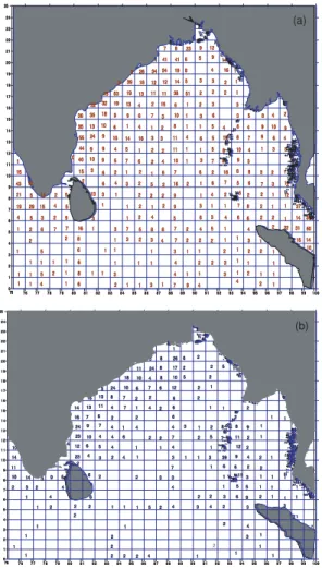
The nitrate profiles for the present study were obtained from the World Ocean Data base 2005 (WOD05) and RNODC. The former contained the nitrate data for the period 1906–1999 while latter had the data for the period 1973–2006. The total number of nitrate profiles extracted from the above sources was 7406. From these the duplicate 10

profiles were removed first and then the rest of the profiles were physically checked for any obvious ambiguity, which was removed subsequently. The quality control pro-cedure reduced the total number of profiles to 2653. The number of profiles available

at each of the 1◦ _latitude

×1◦ longitude grid is shown in Fig. 3a.

The chlorophyll a profiles were taken from RNODC, which contained data for the

15

period 1951–2006. The total number of chlorophyllaprofiles was 1060 and after the

quality control procedure, similar to that of nitrate, the number of profiles reduced to

1030. The number of chlorophyllaprofiles available in each of the 1◦ _latitude

×1◦

lon-gitude grid was shown in Fig. 3b.

Since the total number of nitrate and chlorophyllaprofiles in each of the one-degree

20

grid itself was less, these data were grouped together in time to produce seasonal climatology. The seasons considered for this purpose were defined as:

– Spring intermonsoon March–May

(9)

BGD

10, 16405–16452, 2013

biomass

Title Page

Tables Figures

◭ ◮

Back Close

Full Screen / Esc

Discussion

P

a

per

|

D

iscussion

P

a

per

|

Discussion

P

a

per

|

Discuss

ion

P

a

per

|

– Fall intermonsoon September–October

– Winter monsoon November–February

Since spatial coverage of data during fall intermonsoon was very poor and was con-fined to western Bay of Bengal, this season was not considered.

2.3 River runo_ffdata

5

The monthly mean climatology of river discharge of 6 major rivers Ganges,

Brahma-putra, Irrawady, Godavari, Krishna and Cauvery were taken from Global Runoffdata

Centre, Germany (http://grdc.bafg.de/servlet/is/2781).

2.4 Atmospheric data

Meteorological data were extracted from the National Oceanographic Centre (NOC), 10

Southampton, climatology (formerly Southampton Oceanographic Centre, SOC) (http:

//www.noc.soton.ac.uk/ooc/CLIMATOLOGY/noc11.php) in the study domain (0–25◦_N

and 75–100◦_{E) for the period from 1980 to 2005. It contained the monthly mean}

clima-tology of incoming short wave radiation, wind speed, evaporation, precipitation and net

heat flux on 1◦_{longitude by 1}◦_{latitude grid.}

15

2.5 Remote sensing data

Since the in situ chlorophyll data was limited in both space and time, chlorophyll pig-ment concentrations derived from global 9 km monthly mean imagery of Sea-viewing Wide Field-of-view Sensor (SeaWiFS) for the period September 1997 to Decem-ber 2007 was used (http://reason.gsfc.nasa.gov/OPS/Giovanni/ocean.seawifs.shtml). 20

From these data the climatological seasonal means were calculated for spring inter-monsoon, summer inter-monsoon, fall intermonsoon and winter monsoon.

(10)

BGD

10, 16405–16452, 2013

biomass

Title Page

Tables Figures

◭ ◮

Back Close

Full Screen / Esc

Discussion

P

a

per

|

D

iscussion

P

a

per

|

Discussion

P

a

per

|

Discuss

ion

P

a

per

|

period October 1992 to January 2006, which gives 7 day snapshots having a spa-tial resolution of 1/3rd of a degree, to prepare monthly mean climatology of sea-level anomaly. From the sea-level height anomalies, velocities were computed assuming the geostrophic relation (Pond and Pickard, 1983)

2Ωsin(ϕ)·V =gtan(i) (2)

5

whereΩis the earth’s angular velocity,ϕis the latitude,V is the velocity and tan(i) is

the slope of the sea surface.

3 Results and discussion

We first examined the spatio-temporal variability of mixed layer depth (MLD) by

ana-lyzing the monthly mean climatology. To understand the processes affecting the mixed

10

layer variability we examined the monthly mean climatology of sea surface tempera-ture (SST), sea surface salinity (SSS), incoming short wave radiation, net heat flux (NHF), wind speed (WS), momentum flux (wind-stress curl) and the fresh water flux

(evaporation-precipitation; E-P) in tandem with MLD. For brevity we have presented

the monthly mean climatology of all the above parameters in the Appendix. In the main 15

text we present the monthly mean climatology of MLD superimposed with relevant parameters that are responsible for the observed variability in the mixed layer and dis-cussed the seasonal cycle. Finally, we examine the seasonal variability of chlorophyll and nutrient to understand the possible link between them and mixed layer.

3.1 Spring intermonsoon

20

(11)

BGD

10, 16405–16452, 2013

biomass

Title Page

Tables Figures

◭ ◮

Back Close

Full Screen / Esc

Discussion

P

a

per

|

D

iscussion

P

a

per

|

Discussion

P

a

per

|

Discuss

ion

P

a

per

|

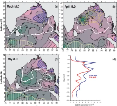
In May, however, the shallow MLD was confined to the region north of 16◦_{N (Fig. 4c).}

Another region of comparatively shallow MLD (∼25 m) was seen in a band between 6◦

and 9◦_{N encompassing peninsular India and Sri Lanka. The rest of the basin, however,}

showed slightly deeper MLD (30–35 m).

The observed MLD variability could be understood in the light of the prevailing 5

ocean-atmospheric conditions. The incoming solar radiation peaked during March–

April (280–290 W m−2_{, Fig. A4) with a corresponding peak in the net heat flux (150–}

160 W m−2_{, Fig. A5). The basin-wide winds were the weakest during this period (4–}

5 m s−1_{, Fig. A6), except near the western boundary in April where a core of high wind}

speed as well as negative wind stress curl was noticed (Fig. 4b). Note that the peak 10

solar heating and subsequent highest net heat gain by the ocean lead to thermal

strat-ification. In addition, low salinity waters in the northern Bay (north of 18◦_{N) with salinity}

less than 32.5 psu (Fig. A3) during March–April lead to strong haline stratification, spe-cially the upper 20 m, as is evident from the vertical profiles of the stability parameter (Fig. 4d). Thus, during spring Intermonsoon the weak winds were unable to break the 15

strong thermohaline stratification to drive deep wind-mixing and hence led to the for-mation of shallow mixed layer.

In the south, comparatively deeper mixed layer (∼35 m) seen west of 90◦E appears

to be linked to the prevailing salinity and wind conditions. The presence of relatively high salinity waters (> 34.5 psu) during spring Intermonsoon (Fig. A3) made the upper 20

water column, specially the upper 30 m, less stable compared to north (Fig. 4d) and the moderate winds (Fig. A6) were able to initiate greater mixing which lead to the observed deep MLD. The comparatively deeper MLD along the western boundary (> 25 m) in

April was driven by the strong negative wind stress curl (∼ −20×10−8Pascal m−1,

Fig. 4b). However, the comparatively shallow MLD in a band between 6◦ _{and 10}◦_N

25

(12)

BGD

10, 16405–16452, 2013

biomass

Title Page

Tables Figures

◭ ◮

Back Close

Full Screen / Esc

Discussion

P

a

per

|

D

iscussion

P

a

per

|

Discussion

P

a

per

|

Discuss

ion

P

a

per

|

3.2 Summer monsoon

Mixed layer during summer monsoon (June-July-August) was the deepest. With the progress of summer monsoon from June to August the mixed layer in most parts of

the Bay and in the region between equator and 6◦_{N was deep (Fig. 5a–c). However,}

along the western boundary and in the northern and eastern part of the Bay MLD was 5

shallow. Similarly, the region around peninsular India and Sri Lanka also showed the presence of shallow mixed layer. With the progress of summer monsoon, the region of shallow mixed layer around Sri Lanka showed a progressive eastward extension with time. The observed pattern of MLD variation could be explained in the follow-ing manner. Though the wind speeds were the highest durfollow-ing summer monsoon in 10

the entire basin (Fig. A6), the MLD were the shallowest in the northern Bay (< 10 m).

An examination of E-P showed that it was negative and the highest of all the

sea-son, implying excess precipitation, in excess of 440 mm month−1_{, in the northern Bay}

(Fig. A8). In addition to the oceanic precipitation, the influx of freshwaters from the rivers adjoining the Bay of Bengal also contributes towards freshening of the surface 15

waters of the Bay. An examination of the monthly mean climatology of river discharge of 5 major rivers Ganges, Brahmaputra, Irrawady, Godavari, and Krishna showed that the freshwater discharge dominated during July to October (Fig. 5d). The spreading of low salinity waters (< 32 psu) were seen from the northern Bay towards the south and also along eastern and western boundary (see the blue cross-hatch in Fig. 5a–c) with 20

the progress of summer monsoon. Note that the upper ocean was very warm with SST

in excess of 28.5◦_{C (Fig. A2). These warm and low salinity waters contributed towards}

strengthening the stratification of the upper ocean as could be inferred from the stabil-ity parameter (Fig. 5e). Thus, though the winds were the strongest of all the seasons, it was unable to break the stratification and initiate wind-driven mixing to deepen the 25

(13)

BGD

10, 16405–16452, 2013

biomass

Title Page

Tables Figures

◭ ◮

Back Close

Full Screen / Esc

Discussion

P

a

per

|

D

iscussion

P

a

per

|

Discussion

P

a

per

|

Discuss

ion

P

a

per

|

stress curl was seen developing in May which peaks in June and collapses by Septem-ber (Fig. A7). This positive wind stress curl drives an upward Ekman pumping and this led to the observed shallow mixed layer around Sri Lanka. The band of deep mixed layer seen extending from the southwestern region of the study area into the central Bay was linked to the advection of high salinity waters from the Arabian Sea. An exam-5

ination of SSS showed progressive advection of high salinity waters from the Arabian Sea into the central Bay during summer monsoon (Fig. A3). This high salinity waters reduced the upper ocean stratification as could be inferred from the stability parame-ter (Fig. 5e). Thus, the strong winds of the summer monsoon combined with the less stratified upper ocean due to the intrusion of high salinity waters from the Arabian Sea 10

were able to drive strong wind-driven mixing. This led to the formation of deep MLD in summer. In addition to this, the negative wind stress curl in the central and western Bay also contributed to the observed deep MLD.

3.3 Fall intermonsoon

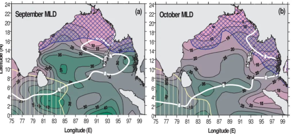
As the summer monsoon tapers offand the fall intermonsoon sets in, the shallow MLD

15

region in the northern Bay, which was confined to north of 18◦_{N, was seen}

extend-ing southward and eastward, while southern part of the Bay showed deep mixed layer (Fig. 6). This could be explained in the context of changing atmospheric forcing from summer monsoon to fall intermonsoon. The short wave radiation as well as net heat flux showed a secondary heating of the upper ocean during fall intermonsoon (Figs. A4 20

and A5) and accordingly the SST was in excess of 29◦_{C in October (Fig. A2). Though}

theE-Pshowed a rapidly decreasing precipitation (Fig. A8) during this period, the

sur-face salinity in contrast showed a progressive decrease from that of summer monsoon (Fig. A3). In addition, the low salinity waters also showed a further southward exten-sion. This indicated that the shallow MLD in the northern Bay and its further southward 25

(14)

BGD

10, 16405–16452, 2013

biomass

Title Page

Tables Figures

◭ ◮

Back Close

Full Screen / Esc

Discussion

P

a

per

|

D

iscussion

P

a

per

|

Discussion

P

a

per

|

Discuss

ion

P

a

per

|

With the setting in of the fall intermonsoon, the winds over the Bay showed a drastic re-duction in their speed in the north (Fig. A6). However, strong winds still persisted in the southern Bay. Thus, the deep MLD in the southern Bay was driven by a combination of comparatively high wind speed and the presence of high salinity waters (Fig. A3) both of which destabilized the water column.

5

3.4 Winter monsoon

The winter monsoon, in general, showed comparatively deep MLD (∼30–40 m) all over

the Bay except in the north and eastern Bay (Fig. 7). The shallow MLD (∼5–15 m) in

the north and eastern Bay could be understood in the context of the presence of low salinity waters (< 32 psu) during November–December (Fig. A3) and associated strong 10

stratification. As the winter progressed, theE-Pshowed a net evaporation in most parts

of the Bay (Fig. A8) while the region of low salinity waters were confined to the northern part during January–February. The shallow MLD observed near the Sumatra coast in January was driven by the strengthened positive wind stress curl (Fig. 7c) and the associated upward Ekman pumping. The deep MLD in the rest of the Bay was related 15

to the weak stratification that occurred in the Bay during winter as could be inferred from the vertical structure of the stability parameter in the upper 40 m (Fig. 7e). The wind speed, which showed a secondary peak in winter (Fig. A6) were able to initiate deeper wind-mixing as the stratification of the water column was the weakest.

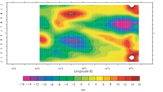
3.5 Role of Rossby waves

20

In order to understand the role of Rossby waves in regulating the MLD the

time-longitude plot of sea-level anomaly along 16◦_{N latitude was analyzed. For this purpose}

the monthly mean climatology of sea-level anomaly was computed from the monthly mean sea-level anomaly data for the period 1992 to 2006.

The time-longitude plot of sea-level anomaly along 16◦_{N showed alternate bands}

25

(15)

BGD

10, 16405–16452, 2013

biomass

Title Page

Tables Figures

◭ ◮

Back Close

Full Screen / Esc

Discussion

P

a

per

|

D

iscussion

P

a

per

|

Discussion

P

a

per

|

Discuss

ion

P

a

per

|

(Fig. 8). These are the signature of westward propagating Rossby waves with positive sea-level anomaly during summer and negative during winter. In summer the central and eastern region showed the highest positive sea-level anomaly and this again con-tributed to the observed deep MLD in the southern Bay in addition to the reduction in stratification due to the intrusion of high salinity waters from the Arabian Sea.

5

3.6 Nitrate and chlorophyll

Having examined the seasonal cycle of basin-scale mixed layer variability, it is impor-tant to analyze the water-column nitrate and chlorophyll to understand how they

re-spond to the changes in the MLD. Towards this, the nitrate and chlorophyllaat 10, 20,

50, and 100 m were analyzed and presented below. Surface values are not presented 10

since the nitrate concentrations are generally in the undetectable levels. Only three seasons namely spring intermonsoon, summer monsoon and winter monsoon were considered as data in the fall intermonsoon was very few as mentioned in Sect. 2.2. In addition, the satellite derived chlorophyll pigment concentrations were also analyzed during the four seasons to decipher the seasonal cycle.

15

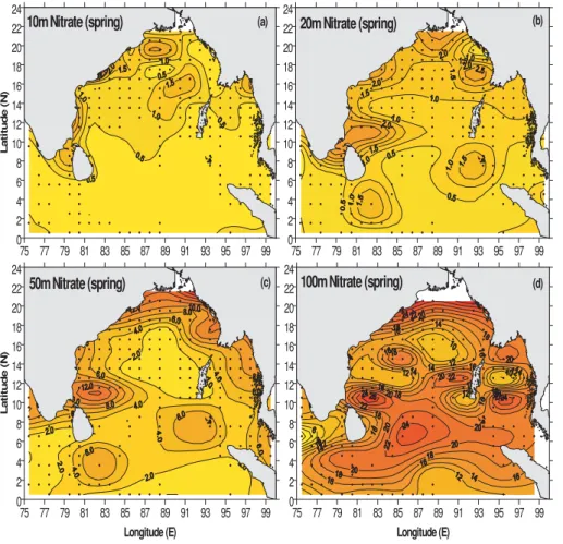
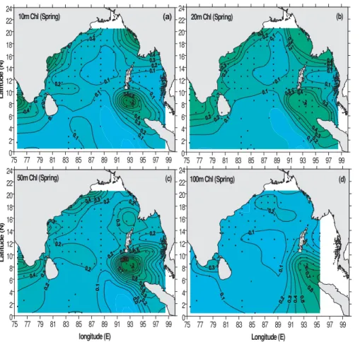
3.6.1 Spring intermonsoon

The nitrate concentrations at 10 m in most part of the basin during spring

intermon-soon was very low ∼0.5 µM (Fig. 9a). Along the northern and western Bay a high

concentration was seen with the values in excess of 1 µM. A large patch in the cen-tral Bay also showed nitrate concentrations in the range of 1 to 1.5 µM. At 20 m, high 20

nitrate concentrations in the range of 1 to 2 µM were seen along the western and north-eastern boundary. The highest concentration of 3 µM was noticed north of Sri Lanka as a patch extending eastward (Fig. 9b). Similarly, two more patches of high nitrate concentration were seen south of Sri Lanka and southeastern Bay respectively. The distribution pattern at 50 m depth was similar to that of 20 m, but concentration levels 25

(16)

concen-BGD

10, 16405–16452, 2013

biomass

Title Page

Tables Figures

◭ ◮

Back Close

Full Screen / Esc

Discussion

P

a

per

|

D

iscussion

P

a

per

|

Discussion

P

a

per

|

Discuss

ion

P

a

per

|

tration showed several eddy-like mesoscale variability and the values varied between 8 and 24 µM (Fig. 9d).

The chlorophyllaconcentration at 10 m during spring intermonsoon was, in general,

less than 0.2 mg m−3_{except near the southern tip of India and along parts of the}

west-ern and eastwest-ern boundary (Fig. 10a). The region between 91 to 98◦_{E and 4 to 10}◦_N

5

also showed highest chlorophyllaconcentrations with maximum value of 0.7 mg m−3_.

In the central and southern Bay the chlorophyll awas least and the value varied

be-tween 0.1–0.2 mg m−3_{. Though the spatial distribution pattern of chlorophyll} _a _{at 20}

and 50 m (Fig. 10b, c) was similar to that of 10 m, the values showed an increase. The

value varied between 0.2–1.0 mg m−3_{. At 100 m the chlorophyll}_a_{concentrations in the}

10

entire Bay was less than 0.2 mg m−3_{except in the southeastern Bay where it showed}

an increase from 0.2 to 0.7 mg m−3_{(Fig. 10d).}

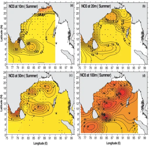
3.6.2 Summer monsoon

The salient feature of nitrate distribution in the upper 20 m during summer was the presence of high concentrations in the Indo-Sri Lankan region where the highest val-15

ues were 6 µM near peninsular India and 3 µM off Sri Lanka (Fig. 11a, b). Another

region of high concentration was in the northern Bay. The rest of the Bay had nitrate concentrations less than 0.5 µM. At 50 and 100 m the eddy-like mesoscale patterns were prominently seen (Fig. 11c, d).

The spatial distribution of chlorophyll a at 10 m showed highest concentration of

20

0.5 mg m−3_{in the northern Bay and also along the western boundary (Fig. 12a).}

How-ever, the pattern was completely different at 20 m and region of highest chlorophyll a

with a value of ∼2 mg m−3 was seen in the Indo-Sri Lanka region (Fig. 12b). In the

rest of the Bay the chlorophyll a concentration was less than 0.2 mg m−3_{. The low}

chlorophyllain the northern Bay in spite of the high nitrate concentration indicates the

25

possible light limitation as the river runoffbrings large amount of suspended load into

(17)

BGD

10, 16405–16452, 2013

biomass

Title Page

Tables Figures

◭ ◮

Back Close

Full Screen / Esc

Discussion

P

a

per

|

D

iscussion

P

a

per

|

Discussion

P

a

per

|

Discuss

ion

P

a

per

|

very low values in the rest of the Bay remained same up to 100 m, their magnitude showed a progressive decrease with depth (Fig. 12c, d).

3.6.3 Winter monsoon

The nitrate distribution at 10 and 20 m (Fig. 13a, b) during winter season showed very

low concentrations in most parts of the Bay (< 0.2 µM), except the region offSumatra.

5

At 50 and 100 m the nitrate concentrations varied between 2 and 24 µM (Fig. 13c, d). The eddy-like mesoscale feature was discernible at these depths.

The chlorophyll a distribution in winter at 10 and 20 m was similar to spring

inter-monsoon, with high values along the western and eastern parts of the Bay, low values

(< 0.1 mg m−3_{) in the rest of the Bay (Fig. 14a, b). At 50 m the chlorophyll} _a _{over the}

10

Bay varied between 0.1 to 0.3 mg m−3_{except along the western boundary where it was}

more than 0.4 mg m−3_{(Fig. 14c). At 100 m most of the Bay showed low chlorophyll} _a

with concentrations of about 0.1 mg m−3_{, except a patch near the southern part of the}

western Bay where the concentration was∼0.5 mg m−3(Fig. 14d).

3.7 Satellite-derived chlorophyll pigment concentrations

15

The satellite-derived chlorophyll pigment concentrations showed the least value during spring intermonsoon compared to the rest of the 3 seasons (Fig. 15). The pigment

concentrations varied over a very narrow range of 0.1 to 0.2 mg m−3_{, except in the}

head Bay and close to peninsular India and Sri Lanka where it marginally increased

to 0.3 mg m−3_{(Fig. 15a). The chlorophyll pigment concentrations during summer}

mon-20

soon were the highest followed by the fall intermonsoon (Fig. 15b, c). The region of highest chlorophyll pigment concentration was located in a region encompassing the peninsular India and Sri Lanka and northern Bay. These patterns were comparable with the in situ concentrations seen in the earlier section. The northern Bay showed

a maximum value of about 1 mg m−3_{, while near the Indo-Sri Lanka region it varied}

25

(18)

BGD

10, 16405–16452, 2013

biomass

Title Page

Tables Figures

◭ ◮

Back Close

Full Screen / Esc

Discussion

P

a

per

|

D

iscussion

P

a

per

|

Discussion

P

a

per

|

Discuss

ion

P

a

per

|

in the pigment concentration map is largely due to sediments and should be neglected. During winter the chlorophyll pigment concentration showed a further reduction from

that of the fall intermonsoon with the values ranging between 0.1 to 0.3 mg m−3_{in most}

parts of the Bay (Fig. 15d). However, close to the western and eastern boundary the

values varied between 0.3 and 2.5 mg m−3_.

5

4 Summary and conclusion

The seasonal variability of mixed layer depth and the factors responsible for the ob-served variability were investigated using a suite of in situ as well as remote sensing data pertaining to ocean and atmospheric parameters. The mixed layer was shallowest during spring intermonsoon compared to the rest of the seasons. The shallow mixed 10

layer in the northern Bay was driven by the strong thermo-haline stratification due to the peak heating by incoming short wave radiation and the presence of low salinity waters. The prevailing weak winds were unable to break the stratification to drive deep wind-mixing resulting in the formation of shallow mixed layer. In the southern Bay, however, the comparatively weaker stratification and the prevalence of moderate winds were able 15

to initiate greater wind-mixing leading to the formation of comparatively deeper mixed layer. During summer, in spite of the fact that the basin-wide winds were the strongest, the northern Bay continued to house shallow mixed layer. The excess precipitation over evaporation combined with the fresh water influx from the rivers adjoining the Bay of Bengal contributed towards freshening of the surface waters of the northern Bay. The 20

resulting strong haline stratification inhibited deep mixing by the strongest winds. The shallow mixed layer in the region encompassing the southern part of the peninsular India and Sri Lanka was due to the upwelling associated with positive wind stress curl, while the band of deep mixed layer extending from southwestern region into the central Bay was associated with the advection of high salinity waters from the Arabian Sea. In 25

(19)

BGD

10, 16405–16452, 2013

biomass

Title Page

Tables Figures

◭ ◮

Back Close

Full Screen / Esc

Discussion

P

a

per

|

D

iscussion

P

a

per

|

Discussion

P

a

per

|

Discuss

ion

P

a

per

|

of annual periodicity also contributed towards the deep mixed layer in the southern Bay. During fall intermonsoon, the south ward extension of the shallow mixed layer resulted from the advection of the low salinity waters from the northern Bay combined with the secondary heating by incoming short wave radiation. The basin-wide deep mixed layer during winter was due to the basin-wide decrease in the upper water column strati-5

fication brought about by a combination of reduced short wave radiation, increase in salinity and comparatively stronger winds.

The seasonal variability of the nitrate and chlorophyll a showed that in the upper

layer the concentration of nitrate was the least during spring intermonsoon compared to the rest of the seasons. The warm and strongly stratified upper ocean during spring 10

intermonsoon with week winds led to shallow mixed layer making it highly oligotrophic.

Consistent with this, the chlorophylla concentrations, both in situ as well as

satellite-derived, were also the least of all the seasons. In contrast, the nitrate concentrations during summer monsoon were the highest in the region encompassing the southern part of the peninsular India and Sri Lanka driven by the wind stress curl. Accordingly, 15

the chlorophyllaconcentrations were also the highest. In the northern Bay though the

nitrate concentrations were high, a concomitant increase was not seen in the

chloro-phyll a indicating the possible light limitation. In fall intermonsoon, though the

nutri-ent data and in situ chlorophylla data were not available, the satellite-derived

chloro-phyll pigment concentrations showed pattern similar to that of summer monsoon with 20

a reduced concentration indicating the tapering effect of summer monsoon. In winter,

though the nitrate concentrations were very low in the upper layers the chlorophylla

concentrations were comparatively high along the western boundary indicating a

mis-match between them. It is to be noted that the number of chlorophylladata for any given

season is much less in comparison with the nitrate data. Also the spatial coverage of 25

chlorophyll a data also is less adequate compared to nitrate data. Hence it is quite

(20)

BGD

10, 16405–16452, 2013

biomass

Title Page

Tables Figures

◭ ◮

Back Close

Full Screen / Esc

Discussion

P

a

per

|

D

iscussion

P

a

per

|

Discussion

P

a

per

|

Discuss

ion

P

a

per

|

high concentrations along the western boundary and the lowest concentrations during spring intermonsooon were all captured. Thus, we see a strong coupling between the seasonal cycle of mixed layer depth and the seasonally altering physical processes which intern is coupled to the chlorophyll pigment concentrations in the upper ocean.

Acknowledgements. Authors are thankful to Direction, CSIR-NIO, Goa and Council of Scientific

5

and Industrial Research (CSIR), New Delhi for all the support and encouragement. We also acknowledge the help rendered by P. M. Muraleedharan, late G. Nampoothiri and M. Nuncio in data collection. This work was supported by Ministry of earth sciences (MoES), New Delhi under the programme BOB Process studies (BOBPS). J. Narvekar acknowledges Department of Science and Technology, New Delhi for the fellowship. This is NIO contribution number xxxxx.

10

References

Bathen, K. H.: On the seasonal changes in the depth of mixed layer in the north Pacific Ocean, J. Geophys. Res., 77, 7138–7150, 1972.

Boyer, T. P., Antonov, J. I.,Garcia, H., Johnson, D. R., Locarnini, R. A., Mishonov, A. V., Pitcher, M. T., Baranova, O. K., and Smolyar, I.: World Ocean Database 2005, Chapter 1:

Introduc-15

tion, NOAA Atlas NESDIS 60, Ed. S. Levitus, US Government Printing Office, Washington, D.C., 182 pp., 2006.

Brainerd, K. E. and Gregg, M. C.: Surface mixed and mixing layer depths, Deep-Sea Res. I., 42, 1521–1543, 1995.

Colburn, J. G.: The thermal structure of the Indian Ocean, International Indian Ocean

Expedi-20

tion Monographs 2, University Press of Hawaii, Honolulu, 1975.

de Boyer Montegut, C., Mignot. J., Lazar, A., and Cravatte, S.: Control of salinity on the mixed layer depth in the world ocean: 1. General description, J. Geophys. Res., 112, C06011, doi:10.1029/2006JC003953, 2007.

Gopalakrishna, V. V., Sadhuram, Y., and Ramesh Babu, V.: Variability of mixed layer depth in

25

the northern Indian Ocean during 1977 and 1979 summer monsoon seasons, Indian J. Mar. Sci., 17, 258–264, 1988.

(21)

BGD

10, 16405–16452, 2013

biomass

Title Page

Tables Figures

◭ ◮

Back Close

Full Screen / Esc

Discussion

P

a

per

|

D

iscussion

P

a

per

|

Discussion

P

a

per

|

Discuss

ion

P

a

per

|

Han, W., McCreary, J. P., and Kohler, K. E.: Influence of precipitation minus evaporation and Bay of Bengal rivers on dynamics, thermodynamics, and mixed layer physics in the upper Indian Ocean, J. Geophys. Res., 106, 6895–6916, 2001.

Kara, A. B., Rochford, P. A., and Hurburt, H. E.: Mixed layer depth variability over the global ocean, J. Geophys. Res., 108, 3079, doi:10.1029/2000JC000736, 2003.

5

Keerthi, M. G., Lengaigne, M. Vialard, J., de Boyer Montégut, C., and Muraleedharan, P. M.: Interannual variability of the Tropical Indian Ocean mixed layer depth, Clim. Dynam., 40, 743–759, 2012.

Levitus, S.: Climatological Atlas of the World Ocean, NOAA Professional paper 13, National Oceanic and Atmospheric Administration, Rockville Md, 173 pp., 1982.

10

Lukas, R. and Lindstrom, E.: The mixed layer of the western equatorial Pacific Ocean, J. Geo-phys. Res., 96, 3343–3357, 1991.

Monterey, G. and Levitus, S.: Seasonal variability of mixed layer depth for the world ocean,

15

NOAA atlas NESDIS 14, US Gov. Printing Office, Washington, D.C., 87 figures & 96 pp., 1997.

Narvekar, J. and Prasanna Kumar, S.: Seasonal variability of the mixed layer in the central Bay of Bengal and associated changes in nutrients and chlorophyll, Deep-Sea Res. I, 53, 820– 835, 2006.

20

Pond, S. and Pickard, G. L.: Introductory dynamical oceanography, Pergamon Press, New York, 241 pp., 1983.

Prasad, T. G.: A comparison of mixed layer dynamics between the Arabian Sea and the Bay of Bengal: One dimensional model results, J. Geophys. Res., 109, C03035, doi:10.1029/2003JC002000, 2004.

25

Rao, R. R., Molinari, R. L., and Festa, J. F.: Evolution of the climatological near-surface ther-mal structure of the tropical Indian Ocean: Description of mean monthly mixed-layer depth and sea-surface temperature, surface-current and surface meteorological fields, J. Geophys. Res., 94, 1081–10815, 1989.

Rao, R. R., Molinari, R. L., and Festa, J. F.: Surface meteorological and near surface

oceano-30

(22)

BGD

10, 16405–16452, 2013

biomass

Title Page

Tables Figures

◭ ◮

Back Close

Full Screen / Esc

Discussion

P

a

per

|

D

iscussion

P

a

per

|

Discussion

P

a

per

|

Discuss

ion

P

a

per

|

Rao, R. R. and Sivakumar, R.: Seasonal variability of near-surface thermal structure and heat budget of the mixed layer of the tropical Indian ocean from a new global ocean temperature climatology, J. Geophys. Res., 105, 995–1016, 2000.

Rao, R. R. and Sivakumar, R.: Seasonal variability of sea surface salinity and salt bud-get of the mixed layer of the north Indian Ocean, J. Geophys. Res., 108, 3009,

5

doi:10.1029/2001JC000907, 2003.

Robinson, M. K., Baur, R. A., and Schroeder, E. H.: Atlas of North Atlantic-Indian Ocean monthly mean temperature and mean salinities of the surface layer, Naval Oceanographic Office Reference Publication 18, Department of the Navy, Washington, D.C, 203073, 213 pp., 1979.

10

Shenoi, S. S. C., Shankar, D., and Shetye, S. R.: Difference in heat budgets of the nearsurface Arabian Sea and Bay of Bengal: Implications for the summer monsoon, J. Geophys. Res., 107, 5-1–5-14, doi:10.1029/2000JC000679, 2002.

Schneider, N. and Muller, P.: The meridional and seasonal structures of the mixed layer depth and its diurnal amplitude observed during the Hawaii-to-Tahiti Shuttle Experiment, J. Phys.

15

Oeanogr., 20, 1395–1404, 1990.

Sprintall, J. and Tomczak, M.: Evidence of barrier layer in the surface layer of the tropics, J. Geophys. Res., 97, 7305–7316, 1992.

Subramanian, V.: Sediment load of Indian Rivers, Cur. Sci., 64, 928–930, 1993.

UNESCO, Technical papers in marine science, United Nations Educational, Scientific and

Cul-20

tural Organization, Paris, 192 pp., 1981.

Vinaychandran, P. N., Murthy, V. S. N., and Ramesh, B. V.: Observations on barrier layer formation in the Bay of Bengal during summer monsoon, J. Geophys. Res., 107, 8018, doi:10:1029/200JC000831, 2002.

Weller, R. A. and Farmer, D. M.: Dynamics of the ocean mixed layer, Oceans, 35, 46–55, 1992.

25

(23)

BGD

10, 16405–16452, 2013

biomass

Title Page

Tables Figures

◭ ◮

Back Close

Full Screen / Esc

Discussion

P

a

per

|

D

iscussion

P

a

per

|

Discussion

P

a

per

|

Discuss

ion

P

a

per

|

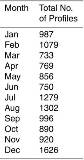
Table 1.Total number of temperature and salinity profiles in the Bay of Bengal for each month

from January to December.

Month Total No.

of Profiles

Jan 987

Feb 1079

Mar 733

Apr 769

May 856

Jun 750

Jul 1279

Aug 1302

Sep 996

Oct 890

Nov 920

(24)

BGD

10, 16405–16452, 2013

biomass

Title Page Abstract Introduction Conclusions References Tables Figures ◭ ◮ ◭ ◮ Back Close

Full Screen / Esc

Printer-friendly Version Interactive Discussion Discussion P a per | D iscussion P a per | Discussion P a per | Discuss ion P a per |

7 6 7 7 7 8 7 9 8 0 8 1 8 2 8 3 8 4 8 5 8 6 8 7 8 8 8 9 9 0 9 1 9 2 9 3 9 4 9 5 9 6 9 7 9 8 9 9 1 0 0 0 1 2 3 4 5 6 7 8 9 1 0 1 1 1 2 1 3 1 4 1 5 1 6 1 7 1 8 1 9 2 0 2 1 2 2 2 3 2 4 4 44 214 62 20 28 11 6 17 14 17 36 9 75 37 17 27 4 19 23 30 55 7 129 39 34 19 24 45 67 37 6 18 16 15 15 11 33 41 42 1 13 13 27 20 14 16 43 27 57 70 40 70 30 25 38 9 37 24 2 47 31 38 7 30 32 41 15 4 13 6 13 11 12 21 32 45 25 48 17 34 28 54 17 7 23 7 10 10 19 15 28 33 41 44 53 32 7 42 43 32 17 16 27 13 6 7 21 21 36 36 53 20 23 40 98 50 37 62 37 11 33 11 11 7 17 16 19 35 47 17 16 17 31 28 27 38 218 18 17 55 37 20 24 12 8 15 31 55 20 25 13 20 43 28 31 31 68 31 32 48 43 20 20 31 20 19 53 66 40 44 11 11 19 33 2 42 39 28 19 39 50 56 30 27 19 27 38 48 159 32 37 168 40 30 35 26 49 51 42 39 57 41 46 63 20 41 27 246 151 35 36 55 34 77 16 57 51 47 48 68 44 64 43 28 33 27 29 30 27 34 28 164 117 154 23 109 19 286 24 53 46 72 61 99 50 31 16 34 29 20 29 11 16 55 48 45 65 12 5 21 10 22 53 67 38 25 28 28 12 18 32 16 18 20 17 30 24 70 13 5 6 13 19 46 53 38 26 42 36 10 14 33 17 6 2 18 18 14 2 9 4 19 2 19 13 32 34 57 47 23 3 1 17 21 18 12 7 20 8 5 6 3 2 17 13 17 9 19 60 31 11 11 28 19 12 19 85 19 2 10 25 18 7 3 3 17 15 8 18 15 18 15 15 17 3 2 8 1 1 12 15 15 8 12 9 10 18 21 19 1 19 14 15 18 19 10 6 11 19 5 1 28 39 32 3 16 15 11 1 75 75 25 25

Fig. 1.Spatial distribution of total number of temperature and salinity profiles available on a 1◦

(25)

BGD

10, 16405–16452, 2013

biomass

Title Page

Tables Figures

◭ ◮

Back Close

Full Screen / Esc

Discussion

P

a

per

|

D

iscussion

P

a

per

|

Discussion

P

a

per

|

Discuss

ion

P

a

per

|

10 12 14 16 18 20 22 24 26 28 30

-200 -180 -160 -140 -120 -100 -80 -60 -40 -20

030 31 32 33 34 35 36 20 21 22 23 24 25 26 27

10 12 14 16 18 20 22 24 26 28 30

-200 -180 -160 -140 -120 -100 -80 -60 -40 -20

028 29 30 31 32 33 34 35 36 17 18 19 20 21 22 23 24 25 26 27

10 12 14 16 18 20 22 24 26 28 30

-200 -180 -160 -140 -120 -100 -80 -60 -40 -20

030 31 32 33- 34 35 36 20 21 22 23 24 25 26

10 12 14 16 18 20 22 24 26 28 30

-200 -180 -160 -140 -120 -100 -80 -60 -40 -20

030 31 32 33 34 35 36 20 21 22 23 24 25 26 27

Density (Kg/m3₎ _{Density (Kg/m}3₎

Density (Kg/m3) Density (Kg/m3)

Salinity (psu)

Salinity (psu) Salinity (psu)

Salinity (psu)

Temperature (°C) Temperature (°C)

Depth (m) Depth (m)

9oN, 89oE 19oN, 89oE

19oN, 89oE 9oN, 89oE

August August

February February

Fig. 2.Vertical profiles of temperature, salinity and density (sigma-t) at two locations

repre-senting the northern (19◦_{N, 89}◦_{E) and southern (9}◦_{N, 89}◦_{E) Bay of Bengal during February}

(26)

BGD

10, 16405–16452, 2013

biomass

Full Screen / Esc

7 6 7 7 7 8 7 9 8 0 8 1 8 2 8 3 8 4 8 5 8 6 8 7 8 8 8 9 9 0 9 1 9 2 9 3 9 4 9 5 9 6 9 7 9 8 9 9 1 0 0 0 1 2 3 4 5 6 7 8 9 1 0 1 1 1 2 1 3 1 4 1 5 1 6 1 7 1 8 1 9 2 0 2 1 2 2 2 3 2 4 1 15 15 43 43 21 21 19 19 4 1 1 1 1 5 29 29 5 2 2 1 1 1 15 15 3 6 5 1 5 4 2 4 2 7 1 2 5 5 5 5 9 7 2 1 1 1 6 8 6 6 8 16 16 2 15 15 40 40 10 10 44 44 55 55 35 35 36 36 1 1 3 13 10 10 9 24 24 13 13 35 35 1 1 3 6 6 9 9 9 10 10 18 18 32 32 2 3 1 1 1 3 1 4 2 5 4 10 10 6 9 19 19 53 53 1 3 7 1 1 3 1 7 5 14 14 1 9 13 13 19 19 39 39 1 1 2 5 2 2 2 2 2 6 1 16 16 4 6 4 13 13 18 18 26 26 3 1 1 8 4 1 2 5 1 2 2 3 1 7 2 11 11 12 12 34 34 14 14 1 4 8 2 2 2 6 4 2 3 2 3 15 15 11 11 12 12 24 24 41 41 7 4 4 3 7 7 5 9 9 16 16 7 10 10 11 11 11 11 8 10 10 6 38 38 14 14 19 19 41 41 9 1 1 2 2 2 1 1 4 1 1 1 1 51 51 5 8 6 23 23 4 1 2 2 1 2 2 4 4 6 6 3 3 1 1 1 1 6 6 3 3 1 1 6 6 1 1 3 3 2 2 2 2 3 3 5 9 9 2 2 2 5 3 1 4 4 6 6 2 2 7 7 5 5 5 5 5 5 6 6 3 3 2 2 4 9 12 12 3 3 3 2 2 1 1 1 1 4 4 1 1 2 7 16 16 8 19 19 4 2 2 16 16 14 14 4 4 1 1 1 1 1 1 6 6 7 7 6 5 5 8 8 9 9 10 10 8 6 6 3 3 1 1 1 1 2 1 2 3 4 6 8 2 6 8 3 4 7 4 5 2 1 2 1 2 2 2 7 3 1 6 9 8 1 1 1 1 1 2 2 1 1 3 2 3 3 6 6 10 10 4 22 22 1 1 12 12 10 10 1 8 4 9 15 15 31 31 14 14 37 37 10 10 14 14 60 60 38 38 1 8 75 75 25 25 3 3 3 1 15 15 3 10 10 15 15 32 32 3 3 7 8 2 1

7 6 7 7 7 8 7 9 8 0 8 1 8 2 8 3 8 4 8 5 8 6 8 7 8 8 8 9 9 0 9 1 9 2 9 3 9 4 9 5 9 6 9 7 9 8 9 9 1 0 0 0 1 2 3 4 5 6 7 8 9 1 0 1 1 1 2 1 3 1 4 1 5 1 6 1 7 1 8 1 9 2 0 2 1 2 2 2 3 2 4 10 10 14 14 11 11 10 10 2 1 14 14 3 1 1 1 2 1 1 9 4 2 5 5 4 4 2 2 2 23 23 12 12 23 23 24 24 16 16 14 14 2 6 6 6 10 10 9 7 13 13 2 3 5 4 7 6 11 11 13 13 2 2 2 1 2 4 4 4 2 4 8 24 24 2 1 4 6 1 7 7 10 10 18 18 2 1 2 1 1 4 2 1 2 6 10 10 11 11 4 5 2 4 2 7 4 24 24 5 2 3 1 2 2 6 8 8 8 4 4 3 7 3 4 7 4 6 6 6 12 12 10 10 17 17 26 26 1 3 5 2 6 1 3 2 2 1 1 2 2 1 1 2 2 2 2 2 4 2 1 1 3 1 1 5 5 2 2 1 2 2 2 2 3 3 1 1 1 6 39 39 7 8 1 1 1 6 6 5 5 11 11 6 9 9 12 12 11 11 8 2 1 1 3 4 3 9 5 3 2 4 2 2 9 2 1 2 1 1 2 2 1 1 1 1 1 1 1 1 1 1 3 1 1 1 1 1 1 1 75 75 25 25 2 4 10 10 3 16 16 1 7 3 4 4 1 2 1 2 5 (a) (b)

Fig. 3.Total number of profiles of(a) nitrate and(b)chlorophylla available at each of the 1◦

(27)

BGD

10, 16405–16452, 2013

biomass

Title Page

Tables Figures

◭ ◮

Back Close

Full Screen / Esc

Discussion

P

a

per

|

D

iscussion

P

a

per

|

Discussion

P

a

per

|

Discuss

ion

P

a

per

|

75 77 79 81 83 85 87 89 91 93 95 97 99 0

2 4 6 8 10 12 14 16 18 20 22 24

La

ti

tude

(

N

)

March MLD (a)

75 77 79 81 83 85 87 89 91 93 95 97 99

Longitude (E)

0 2 4 6 8 10 12 14 16 18 20 22 24

La

ti

tude

(

N

)

May MLD (c)

75 77 79 81 83 85 87 89 91 93 95 97 99 0

2 4 6 8 10 12 14 16 18 20 22 24

April MLD (b)

0 1 2 3 4 5 6 7 8 910 Stability parameter (x10-5) -220

-200 -180 -160 -140 -120 -100 -80 -60 -40 -20 0

D

e

pt

h (

m

)

20o_{N, 88}o_E 7o_{N, 88}o_E

(d)

Fig. 4.Monthly mean climatology of mixed layer depth (m) in the Bay of Bengal during spring

intermonsoon(a)March,(b)April and(c)May, and(d)vertical profiles of upper ocean stability parameter (E, m−1_{) at 20}◦_{N, 88}◦_{E (blue line) and 7}◦_{N, 88}◦_{E (red line) in April. In} _(a–c) _the

(28)

BGD

10, 16405–16452, 2013

biomass

Full Screen / Esc

75 77 79 81 83 85 87 89 91 93 95 97 99 0 2 4 6 8 10 12 14 16 18 20 22 24 La ti tu de ( N )

June MLD (a)

75 77 79 81 83 85 87 89 91 93 95 97 99 0 2 4 6 8 10 12 14 16 18 20 22 24

July MLD (b)

75 77 79 81 83 85 87 89 91 93 95 97 99

Longitude (E) 0 2 4 6 8 10 12 14 16 18 20 22 24 La ti tude ( N )

August MLD (c)

1 2 3 4 5 6 7 8 9 10 11 12

Month 0 5000 10000 15000 20000 25000 30000 35000 40000 45000 50000 Ri v e r Di s c h a rg e ( m 3/s ) Brahmaputra Ganges Irrawady Godavari Krishna (d)

0 10 20 30 40 50

Stability parameter (x10-5) -220 -200 -180 -160 -140 -120 -100 -80 -60 -40 -20 0 D e pt h ( m )

18o_{N, 88}o_E

7o_{N, 88}o_E

(29)

BGD

10, 16405–16452, 2013

biomass

Title Page

Tables Figures

◭ ◮

Back Close

Full Screen / Esc

Discussion

P

a

per

|

D

iscussion

P

a

per

|

Discussion

P

a

per

|

Discuss

ion

P

a

per

|

Fig. 5.Monthly mean climatology of mixed layer depth (m) in the Bay of Bengal during summer

(a) June,(b) July and (c) August, (d) monthly mean river discharge climatology of Ganges, Brahmaputra, Irrawady, Godavari and Krishna and(e)vertical profiles of upper ocean stability parameter (E, m−1_{) at 18}◦_{N, 88}◦_{E (blue line) and 7}◦_{N, 88}◦_{E (red line) in the Bay of Bengal}

(30)