GABRIELLE FERREIRA PIRES
CLIMATE CHANGE AND THE SUSTAINABILITY OF AGRICULTURAL PRODUCTIVITY IN BRAZIL
Tese apresentada à Universidade Federal de Viçosa, como parte das exigências do Programa de Pós-Graduação em Meteorologia Aplicada, para obtenção do título de Doctor Scientiae.
VIÇOSA
ii À minha mãe Margarida Ferreira Pires.
iii “Não seja o de hoje.
Não suspires por ontem.... Não queiras ser o de amanhã. Faze-te sem limites no tempo. ”
iv ACKNOWLEDGMENTS
À Deus, por tantas bênçãos em minha vida e por dar-me força, proteção, sabedoria e saúde.
À minha mãe Margarida, ao meu pai Tarcísio e à minha irmã Monique pela compreensão, pelo amor incondicional, pelo apoio constante, pelos ensinamentos e incentivos e por toda a confiança depositada em mim.
Ao meu marido e melhor amigo Ulisses (Uli), por todo o amor e leveza, pela fortaleza e proteção, pelo essencial incentivo e apoio nas horas de dificuldade, pela dedicação, pelos exemplos de pessoa e de caráter.
Ao meu orientador, Professor Marcos Heil Costa, me faltam palavras para agradecer todos os ensinamentos e oportunidades de aprendizagem que me foram proporcionadas durante a carreira científica. Prof. Marcos é meu grande exemplo de cientista e dedicação à docência, e fez-me fascinar pela carreira. Agradeço imensamente pela amizade, por toda a confiança depositada em mim, pelos ensinamentos preciosos, pelo apoio profissional e pessoal, pelos exemplos de profissionalismo e competência. O sentimento é de profunda gratidão e admiração.
Ao Gabriel e à Livia Brumatti, agradeço por toda a ajuda, amizade, dedicação e pró-atividade. Foram muito valiosas a convivência e a troca de experiências. Aprendi muito com vocês nesses anos, e sem vocês esta jornada não teria sido a mesma.
Aos demais colegas do Grupo de Pesquisas em Interação Atmosfera-Biosfera da UFV, Lívia, Pauline, Vítor, Emily, Aninha, Raphael, Fabiana, Carol, Matheus, Telmo, Fernando, Argemiro, Hewlley, Carla, Leydimere, Marcos Paulo, Ana Cláudia e Richard, pela agradável convivência e por toda a ajuda, incentivos, disponibilidade e parceria.
v Agradecimentos especiais a Victor Brovkin (Max Planck Institute), Chris Jones e Spencer Liddicoat (Hadley Centre), e Etsushi Kato (The Institute of Applied Energy, Japan) por toda a atenção e pela ajuda com os dados do experimento LUCID.
Ao Milton Pereira e sua equipe de coleta dos dados relativos ao cultivo de
Brachiaria Brizantha, pelo fornecimento dos dados.
À Universidade Federal de Viçosa e ao Departamento de Engenharia Agrícola pela
oportunidade de concluir o Doutorado em Meteorologia Aplicada.
Ao Conselho Nacional de Desenvolvimento Científico e Tecnológico (CNPq),
pela concessão de bolsa de estudos. À Fundação Gordon and Betty Moore (Moore
Foundation), pelo apoio financeiro.
A todos os professores do programa de pós-graduação em Meteorologia Agrícola/Aplicada, pelos conhecimentos transmitidos.
À Graça, excelente secretária da Meteorologia Aplicada/Agrícola, pela ajuda e amizade ao longo do Doutorado.
vi BIOGRAPHY
GABRIELLE FERREIRA PIRES, filha de Sebastião Tarcísio Pires e Margarida Ferreira Pires, nasceu em 02 de janeiro de 1987, na cidade de Belo Horizonte - MG.
Iniciou a graduação em Engenharia Ambiental em março de 2005, obtendo o título de Engenheira Ambiental em janeiro de 2010 pela Universidade Federal de Viçosa (UFV).
Em fevereiro de 2012 concluiu o mestrado em Meteorologia Agrícola na Universidade Federal de Viçosa (UFV).
vii CONTENTS
LIST OF FIGURES ix
LIST OF TABLES xi
LIST OF SYMBOLS xii
LIST OF ACRONYMS xiv
RESUMO xvi
ABSTRACT xviii
GENERAL INTRODUCTION 1
CHAPTER 1 INCREASED CLIMATE RISK IN BRAZILIAN DOUBLE CROPPING AGRICULTURE SYSTEMS UNTIL 2050 AND IMPLICATIONS FOR LAND USE
IN NORTHERN BRAZIL 6
1.1 INTRODUCTION 6
1.2 MATERIALS AND METHODS 10
1.2.1 Productive regions 10
1.2.2 Climate models and input data 12
1.2.3 Crop model description 16
1.2.4 Experiment design 17
1.3 RESULTS AND DISCUSSION 24
1.3.1 Effects of climate change in ESOY and HSOY productivity 24 1.3.2 Implications for double-cropping systems in central-northern Brazil 31
1.4 CONCLUSIONS 35
CHAPTER 2 EFFECTS OF CLIMATE CHANGE IN PASTURE PRODUCTIVITY
AND IMPLICATIONS FOR LAND USE IN BRAZIL 39
2.1 INTRODUCTION 39
viii
2.2.1 Productive regions 41
2.2.2 Climate models and input data 43
2.2.3 Pasture model description 44
2.2.4 Experiment design 46
2.3 RESULTS 47
2.4 DISCUSSION AND CONCLUSIONS 51
CHAPTER 3 GENERAL CONCLUSIONS 55
3.1 THESIS OVERVIEW 55
3.2 CONCLUSIONS 57
3.3 RECOMMENDATIONS FOR FUTURE RESEARCH 61
GENERAL REFERENCES 63
ix LIST OF FIGURES
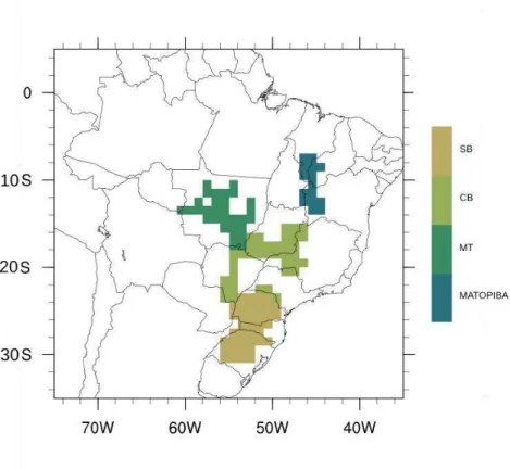
Figure 1.1 – Analyzed productive regions. Each 1o x 1o pixel shown here had at least 10% of its area planted with soybean in 2012 according to Dias et al. (submitted).
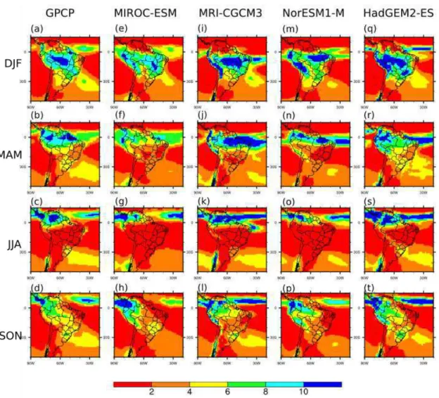
11 Figure 1.2 - Daily mean precipitation (mm/day) for the period 1979-2000 during the phases of the South American Monsoon System (SAMS). Data is shown for Global Precipitation Climatology Project data (GPCP) (a-d) and simulated by MIROC-ESM (e-h), MRI-CGCM3 (i-l), NorESM1-M (m-p) and
HadGEM2-ES (q-t). 14
Figure 1.3 ‒ Daily mean precipitation for each month of the period 1979-2000 as in Global Precipitation Climatology Project (GPCP) and as simulated by the models: MIROC-ESM, MRI-CGCM3, NorESM1-M and HadGEM2-ES. The monthly averages are calculated over each one of the soybean productive regions in Brazil (Figure 1.1). The average results of the model ensemble is also shown
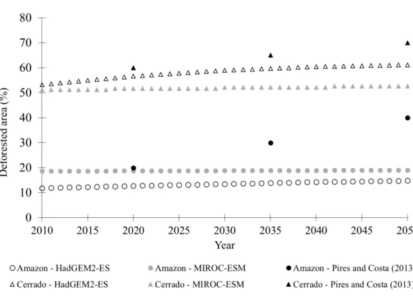
15 Figure 1.4 – Scenarios of total Amazon and Cerrado deforested area according to RCP8.5 as implemented in models HadGEM2-ES and MIROC-ESM and to Pires and
Costa (2013). 23
Figure 1.5– Percentage change in soybean yield from 2011-2020 to 2041-2050 after climate change. In (a) and (b) atmospheric composition and land use trajectories
are according CMIP5’s RCP8.5 scenario. In (c) and (d), atmospheric composition trajectories are according to CMIP5’s RCP8.5 scenario, but land
use trajectories are according to Pires and Costa (2013) tropical deforestation
scenarios. 27
x (triangles and dashed lines are the average and the models range, respectively).
30 Figure 1.7 – Soybean productivity change [Yd(2041-2050) / Y09/25(2011-2020), where d are the planting dates assessed in this study] after climate change. Full black boxes (circles) represent soybean planting dates that lead to a high probability of double-cropping viability according to RCP8.5 (LUCID+PC13). Full gray boxes (circles) represent soybean planting dates that lead to a medium probability of double-cropping viability, also according to RCP8.5 (LUCID+PC13). Empty boxes (circles) represent soybean planting dates that may lead to unviable double-cropping according to RCP8.5 (LUCID+PC13).
Dashed boxes indicate the sowing windows. 34
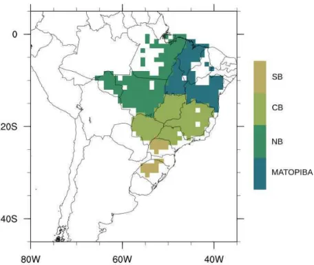
Figure 2.1 – Analyzed productive regions. Each 1o x 1o pixel shown here had at least 10%
of its area covered by pasturelands in 2012. 42
Figure 2.2 – Daily mean precipitation for each month of the period 1979-2000 as in GPCP and as simulated by the models: MIROC-ESM, MRI-CGCM3, NorESM1-M and HadGEM2-ES. The monthly averages are calculated over each one of the
soybean productive regions in Brazil. 44
Figure 2.3 – Percentage change in pasture productivity from 2011-2020 to 2041-2050 after climate change. In (a) atmospheric composition and land use trajectories are
according CMIP5’s RCP8.5 scenario. In (b) atmospheric composition
trajectories are according to CMIP5’s RCP8.5 scenario, but land use trajectories
are according to Pires and Costa (2013) tropical deforestation scenarios. 49 Figure 2.4 – Change in yearly precipitation (mm/yr) from 2011-2020 to 2041-2050 after climate change to the most productive Brazilian regions, as in RCP8.5 (circles and solid lines are the average and the models range, respectively) and LUCID+PC13 5 (triangles and dashed lines are the average and the models
xi LIST OF TABLES
Table 1.1 – Main soybean productive regions in Brazil and their total production. Data for Brazilian states are from IBGE (2015). Total Brazilian production in 2014 is
~8.68x10⁷ ton. 11
Table 1.2 – List of CMIP5 models used in this study 13 Table 1.3 – Change in soybean productivity from 2011-2020 to 2041-2050 for different Brazilian productive regions, for short cultivars (1600 GDD) planted in Sep 25th (ESOY). In the second column, both atmospheric composition and land-use change trajectories are according to RCP8.5. In the third column, atmospheric composition is according to RCP8.5 and land use change is
according to (Pires and Costa, 2013). 28
xii LIST OF SYMBOLS
Cdf ‒ final daily climate input (emission + land use change scenario) Cd ; LUCID ‒ daily LUCID climate variable
Cm ; A10C60‒ monthly mean climate for A10C60 Pires and Costa (2013) scenario
Cm ; scenario‒ monthly mean Pires and Costa (2013) climate variable (A20C60 from 2009 to 2020; A30C65 from 2021 to 2035; A40C70 from 2036 to 2050)
ESOY ‒ Early soybean cultivar (average cycle duration of 100 days) planted right after the end of the sanitary break (September 25th)
HSOY ‒ Highly productive soybeans
LUCID+PC13 ‒ Climate change scenario which assumes that climate change leads to a radiative forcing of about 8.5 Wm- 2 in 2100, but deforestation scenarios are as Pires and
Costa (2013)
P ‒ Pasture productivity
P2011-2020 ‒ Average pasture productivity in 2011-2020 P2041-2050 ‒ Average pasture productivity in 2041-2050 PC13 ‒ Deforestation scenarios from Pires and Costa (2013)
RCP8.5 ‒ Climate change scenario which assumes that climate change leads to a radiative forcing of about 8.5 Wm- 2 in 2100
Y ‒ Soybean productivity
xiii YMAXLUCID+PC13 ‒ HSOY productivity under the RCP8.5 scenario
xiv LIST OF ACRONYMS
CB – Central Brazil
CMIP5 – Coupled Model Intercomparison Project Phase models 5 COP – Conference pf the Parties
EMBRAPA – Empresa Brasileira de Pesquisa Agropecuária ESM – Earth System Model
FAO – Food and Agriculture Organization GCM – Gridded Crop Models
GDD – Growing Degree-Days GDP – Gross Domestic Product
GPCP – Global Precipitation Climatology Project data
HadGEM2-ES – Hadley Centre Global Environmental Model, version 2 IBGE – Brazilian Institute of Geography and Statistics.
IBIS – Integrated Biosphere Simulator
INLAND – Integrated Model of Land Surface Processes INDC - intended Nationally Determined Contribution
IPCC AR5 – Intergovernmental Panel on Climate Change – Assessment Report #5
ITCZ – Inter Tropical Convergence Zone LAI – Leaf Area Index
xv MATOPIBA – Maranhão, Tocantins, Piauí and Bahia
MT – Mato Grosso
MIROC-ESM – Model for Interdisciplinary Research on Climate
MRI-CGCM3 – the Meteorological Research Institute Coupled Atmosphere–Ocean General Circulation Model, version 3
NB – Northern Brazil
NorESM1-M – Norwegian Earth System Model, version 1 PFT – Plant Functional Type
PPCDAm – Plano de Ação para Prevenção e Controle do Desmatamento na Amazônia Legal
PPCerrado – Plano de Ação para Prevenção e Controle do Desmatamento e das Queimadas no Cerrado
PRODES – Projeto de Monitoramento da Floresta Amazônica Brasileira por Satélite SACZ – South Atlantic Convergence Zone
xvi RESUMO
PIRES, Gabrielle Ferreira, D.Sc., Universidade Federal de Viçosa, dezembro de 2015. Mudanças climáticas e a sustentabilidade da produtividade agrícola no Brasil. Orientador: Marcos Heil Costa.
xviii ABSTRACT
PIRES, Gabrielle Ferreira, D.Sc., Universidade Federal de Viçosa, December, 2015. Climate change and the sustainability of agricultural productivity in Brazil. Adviser: Marcos Heil Costa.
1 GENERAL INTRODUCTION
Historically, agribusiness is one of the pillars of Brazilian economy, representing 20-30% of its Gross Domestic Product (GDP) (CEPEA, 2014). Initially, Brazil was a producer of large monocultures such as sugarcane and coffee, but diversified its production and became the third largest agricultural exporter in 2010 (WTO, 2010), exporting meat, fruit, grains and cereals. Brazil became a world leader in meat exportation, but consequently replaced the Cerrado and Amazonia biomes by pasture (Leite et al., 2012). The country is also a leader in soybean production, expanding farms from the Southern region to Cerrado, and more recently, Amazonia.
2 future development of world agriculture, predicted that Brazil will have the largest increase in planted area in the world until 2050.
It is clear that the increasing population and consumption will place unprecedented demands on agriculture and natural resources (Foley et al., 2011). However, if a significant part of the increase in agricultural production in Brazil occurs by expanding the agriculture frontier and degrading biomes, we run a great risk. Recent studies indicate that large-scale deforestation drives significant changes in water availability and could have strong implications for agricultural production systems and food security in some regions (Lawrence and Vandecar, 2015). Simulations show that the replacement of forest or savanna by crops and pastures can cause a regional climate change mainly characterized by significant reductions in local precipitation (Sampaio et
al., 2007; Costa et al., 2007; Walker et al., 2009; Pires and Costa, 2013) and increased dry
season length (Costa and Pires 2010).
3 On the other hand, the pressure to reduce the Amazon deforestation rates has increased both nationally and internationally, and the levels of deforestation in Amazonia unprecedentedly decreased 77% from 2005 to 2011 when compared to 1995 to 2005 rates (Nobre, 2012, PRODES 2015, Hansen et al., 2013), despite the high meat and soybean prices in the international market. This reduction in the Amazon deforestation rates was a consequence of a number of factors: state and federal governance, increased surveillance and the voluntary adoption of soybean and meat moratorium (Boucher, 2014). However, most of the curbed deforestation in the Amazon leaked to the Cerrado biome, the world richest savanna in biodiversity and the main agriculture hotspot in Brazil, where conservation policies are weak (Gibbs et al., 2015).
Nevertheless, subsequently to 8 years of dramatic reductions in Amazon deforestation rates, in 2013 the decreasing trends reversed and started to increase again until 2015, according to PRODES (Projeto de Monitoramento da Floresta Amazônica
Brasileira por Satélite). This increase in deforestation rates may also be related to the
revision of the Forest Code in 2012, that according to Soares-Filho et al. (2014), may allow additional deforestation. Gibbs et al. (2015) also argue that, with the end of Soy Moratorium by May 2016, Federal enforcement mechanisms are unlikely to effectively keep low deforestation levels in the soy supply chain. Therefore, currently there is little evidence that agriculture expansion is coming to a halt in Cerrado and Amazonia (Bowman et al., 2012; Lapola et al., 2014).
4 change induced by the change in atmospheric composition, hereafter referred to as global climate change. This type of climate change leads to a warming of the surface and is also predicted to change precipitation patterns, especially during the dry season (Malhi et al., 2008; Fu et al., 2013). On the other hand, besides the radiative effects of carbon dioxide (CO2) as a greenhouse gas, there is also an additional effect on the vegetation physiological processes as higher atmospheric CO2 concentrations may stimulate canopy photosynthesis and decrease stomatal conductance (Sellers et al., 1996), increasing water use efficiency, especially in C3 plants (as soybeans). However, according to Clark (2004), the increased temperature and drought may limit these positive physiological effects related to increased atmospheric CO2 concentration. Despite the scenario of global climate change, strong negative effects are expected across the globe, especially higher levels of warming at low latitudes (Rosenzweig et al., 2014).
6 CHAPTER 1
INCREASED CLIMATE RISK IN BRAZILIAN DOUBLE CROPPING AGRICULTURE SYSTEMS UNTIL 2050 AND IMPLICATIONS FOR LAND
USE IN NORTHERN BRAZIL
1.1 INTRODUCTION
Brazil is the second largest soybean producer and the third largest maize producer in the world, contributing with 30% and 7%, respectively, of the global harvest of these crops in 2013. While global production of these commodities nearly doubled from 1993 to 2013, Brazil soybean and maize production increased three-fold. This increase in production in the last 20 years is greater than the increase observed in the United States, the main producer of these commodities worldwide (FAO, 2015).
A great share of the dramatic increase in grain production during the last decade in Brazil was possible due to the extensive adoption of double-cropping systems, in which farmers sow a second crop (mainly maize, but cotton is also common) in the same space after soybean has been harvested. The second crop production was not relevant until a decade ago, but in 2014 it represented nearly 58% of the total maize harvested area, thanks to the expressive technological progress that took place in the main productive regions in the country (CONAB, 2015).
7 In some productive regions in the country, the rainy season is about 6-7 months long and in order to the double-cropping system to be agronomically viable, it is necessary to anticipate soybean cycle so that it is harvested in time for the second crop to grow, flower and fill grains while climatic conditions (precipitation and temperature) are still favorable, or more specifically, before the rainy season ends. Therefore, considering that the sowing operation may be as long as 2 to 4 weeks since central-northern Brazilian soybean ranch may be as extensive as 10,000 ha, farmers who aspire to use double-cropping systems typically choose to sow early soybean cultivars and as soon as possible, right after the end of the sanitary break, when rainfall conditions are just marginally favorable in central Brazil.
The sanitary break, adopted by Brazil and Paraguay, is a 2-3 month period of absence of living soybean plants in the field, as a measure to control infection with Asian soybean rust (Phakopsora sp), and typically lasts from June 15 to September 15or 30 in Brazil. In the case of sowing soybean at the end of the sanitary break, even though climate risk is relatively high, sanitary risk is small since the probability of infection with rust is still low and early crops remain less time in the field exposed to infection. Another incentive for farmers is the higher market prices for soybean harvested earlier than in the peak of the harvesting season.
8 Brazilian Ministry of Agriculture, Livestock and Supply (MAPA, from the acronym in Portuguese) estimates that the production of these commodities will increase 33.9% and 26.3%, respectively, mainly for exportation. In order to be sustainable, the potential increase in food production in Brazil must not rely on a proportional increase in cultivated area (Foley et al., 2011), and double-cropping systems might play an important role to achieve this objective.
While total grain production is expected to increase, recent long-term climate forecasts indicate potential unfavorable climate conditions in Brazilian productive regions. The dry season in southern Amazonia may be becoming longer (Butt et al., 2011; Costa and Pires, 2010; Fu et al., 2013), due to both deforestation and the change in atmospheric composition, and such evolution may be incompatible with the adoption of double-cropping systems (Arvor et al., 2014).
9 role of adaptation of planting dates and cultivars in response to climate change. Rosenzweig et al. (2014) assessed the change in agricultural productivity in the global scale, but used either fixed planting dates and cultivars or methods to estimate these parameters according to favorable climatic conditions, therefore failing to represent
farmers’ decision to sow soybeans under unfavorable climatic conditions to plant two
crops in the same agricultural calendar.
Brazilian agriculture, however, is more complex, and in addition to recommended planting dates and cultivars that lead to high productivity, higher levels of profit are also
determined by important aspects as the farmer’s choice to plant one or more crops in the
same space in the same crop year, and the low incidence of plant diseases. Although important, the large-scale aspects of these features are understudied for Brazil and a more realistic estimate of a change in soybean yield under climate change scenarios, that also
includes farmer’s choice and the incidence of disease, is still missing.
Here we examine these patterns by using one gridded crop model and four climate models to assess how regional and global climate change may affect soybean productivity until 2050 under the following management practices, which aim to represent realistic scenarios:
(i) farmers who choose to plant early soybean cultivars immediately after the end of the sanitary break to plant two crops in the same agricultural calendar; (ii) farmers who choose to plant only one crop in the agricultural calendar, and
10 The results presented here may be critical to create effective solutions to mitigate the negative effects of climate change in soybean productivity and to maintain high levels of production in the productive regions.
1.2 MATERIALS AND METHODS
1.2.1 Productive regions
We evaluated individually the results of soybean productivity change in the main productive regions in Brazil (Figure 1.1), identified by the following acronyms: Mato Grosso (MT); MATOPIBA, which aggregates results for Maranhão, Tocantins, Piauí and Bahia states; Central Brazil (CB), with results from Mato Grosso do Sul, Goiás, Minas Gerais and São Paulo states; and Southern Brazil (SB), for Paraná, Santa Catarina and Rio Grande do Sul. Together, these regions produce 98% of the soybean produced in Brazil in 2014 (IBGE, 2015 - Table 1.1).
In all Brazilian productive regions, we used the soybean planted area from Dias et
al. (submitted) to filter the pixels that have at least 10% of its area planted with soybeans
11 Figure 1.1 – Analyzed productive regions. Each 1o x 1o pixel shown here had at least 10% of its area planted with soybean in 2012 according to Dias et al. (submitted).
Table 1.1 – Main soybean productive regions in Brazil and their total production. Data for Brazilian states are from IBGE (2015). Total Brazilian production in 2014 is ~8.68x10⁷ ton.
Region Acronym Production in 2014
(ton)
% from total Brazilian production in 2014
Maranhão, Tocantins,
Piauí and Bahia MATOPIBA
8.66 x 10⁶ 9.99
Mato Grosso MT 26.5 x 10⁶ 30.54
Central Brazil CB 20.3 x 10⁶ 23.43
Southern Brazil SB 29.6 x 10⁶ 34.14
12 1.2.2 Climate models and input data
With the objective to select suitable Climate/Earth System Models to represent future climate, we chose to evaluate simulated historical precipitation, since this is one of the most poorly simulated physical processes in Earth System Models (ESMs) (Flato et
al., 2013), and is determinant to rainfed agriculture productivity.
Here we assess the historical simulations (1979-2000) of four global models from the Coupled Model Intercomparison Project Phase models 5 - CMIP5 (Taylor et al., 2012) that contributed to the Intergovernmental Panel on Climate Change Fifth Assessment Report (IPCC AR5) (Table 1.2). The seasonal climatology of simulated precipitation over South America for the last 21 years of the 20th century (1979 to 2000) was evaluated based on the Global Precipitation Climatology Project data (GPCP) (Adler et al., 2003).
13 models seem to slightly underestimate precipitation in central-Brazil. MIROC-ESM and NorESM1-M also underestimate precipitation for Southern regions, but HaGEM2-ES and MRI-CGCM3 seem to represent it well.
According to the precipitation annual cycle for soybean productive regions (Figure 1.3), virtually all models represent well the season cycle, even though the magnitude of simulated precipitation varies among models.
Table 1.2 – List of CMIP5 models used in this study
Model name Acronym Institute
Model for Interdisciplinary Research on Climate, version
5
MIROC-ESM
Atmosphere and Ocean Research Institute (The University of Tokyo),
National Institute for Environmental Studies, and
Japan Agency for Marine-Earth Science and
Technology Meteorological Research
Institute Coupled Atmosphere–Ocean General
Circulation Model, version 3 MRI-CGCM3
Meteorological Research Institute (MRI), Japan
Norwegian Earth System Model, version 1 (medium
resolution)
NorESM1-M Norwegian Climate Centre (NCC)
The Hadley Centre Global Environmental Model,
version 2
14 Generally, models underestimate precipitation in comparison to GPCP in nearly all months of the seasonal cycle. From all models, HadGEM2-ES has the best performance and is reasonably closer to GPCP, although it slightly overestimates precipitation from June to January.
15 Figure 1.3‒ Daily mean precipitation for each month of the period 1979-2000 as in Global Precipitation Climatology Project (GPCP) and as simulated by the models: MIROC-ESM, MRI-CGCM3, NorESM1-M and HadGEM2-ES. The monthly averages are calculated over each one of the soybean productive regions in Brazil (Figure 1.1). The average results of the model ensemble is also shown
Besides precipitation (mm/day), the climate variables used as input to INLAND simulations are specific humidity (kgH2O/kg air), solar radiation (W/m2), average wind speed (m/s) and average, maximum and minimum temperatures (oC).
0 2 4 6 8 10 12 14 Ja n Feb Ma r A pr Ma y
Jun Jul Aug Sep Oct Nov Dec (b) MT 0 2 4 6 8 10 12 14 Ja n Feb Ma r A pr Ma y
Jun Jul Aug Sep Oct Nov Dec (c) CB GPCP Ensemble 0 2 4 6 8 10 12 14 Ja n Feb Ma r A pr Ma y
Jun Jul Aug Sep Oct Nov Dec (d) SB NorESM1-M HadGEM2-ES MRI-CGCM3 MIROC-ESM 0 2 4 6 8 10 12 14 Ja n Feb Ma r A pr Ma y
16 1.2.3 Crop model description
We use a mechanistic gridded crop model (GCM) to evaluate the change in soybean productivity after climate change: the Integrated Model of Land Surface Processes (INLAND, Costa et al., in prep.).
INLAND is a fifth-generation land surface model that simulates the exchanges of energy, water, carbon and momentum in the soil-vegetation-atmosphere system, the canopy physiology (photosynthesis, stomatal conductance and respiration) and the terrestrial carbon balance (net primary productivity, soil respiration and organic matter decomposition). Total carbon assimilation is allocated to leaf, stem, root or grains depending on the phenological stage. More specifically, the allocation scheme considers three phenological stages controlled by Growing Degree-Days (GDD): (i) from planting to leaf emergence; (ii) from leaf emergence to end of silking; (iii) from grain fill to physiological maturity. Soybean productivity is estimated based on the percentage of dry matter allocated to grains. Processes are organized in a hierarchical framework, and operate in time-steps of 60-min. This model is an evolution of Agro-IBIS (Integrated Biosphere Simulator) (Kucharik and Twine, 2007) and has been developed by Brazilian researchers as part of the Brazilian Earth System Model project, aiming to better represent biomes (as Amazon and Cerrado) and processes (as fire, flooding and agriculture) that take place in Brazilian territory. We use the version 2.0, which includes the representation of four crops, in addition to 12 natural plant functional types.
17 1.2.4 Experiment design
1.2.4.1 Planting dates and cultivars
In each individual simulation in this work (sets of simulations are described in section 1.2.4.2) we simulated 10 planting dates (09/15, 09/25, 10/05, 10/15, 10/25, 11/05, 11/15, 11/25, 12/05 and 12/15) and 5 cultivars, that vary according to the accumulation of growing degree-days (GDD) needed to achieve physiological maturity - from the shortest to the longest cultivar: 1500, 1600, 1700, 1800 and 1900 GDD (base temperature 10oC), with typical total cycle duration from 100 to 130 days. Therefore, for every model/scenario considered in this study, we have 50 possible configurations of planting dates and cultivars for each pixel. We then focus our analysis on two specific cases:
ESOY: Short-cycle soybean cultivar (average cycle duration of 100 days) planted
early right after the end of the sanitary break (September 25th), to represent farmers who choose to harvest soybean in time to plant a second crop in the same agricultural calendar;
HSOY: Highly productive soybeans, representing farmers who choose to plant only
18 1.2.4.2Land use and climate change scenarios
We conducted two sets of simulations, from 2011 to 2050, to estimate the change in soybean productivity after climate change, as follows.
Effects of land-use change and change in atmospheric composition on climate as in
CMIP5 (RCP8.5)
This group of simulations accounts for the effects of land-use change and the change in atmospheric composition on climate with both land use and atmospheric composition according to the CMIP5 (Coupled Model Intercomparison Project Phase 5) experiment. Here we assess the RCP 8.5 W.m-2 scenario (RCP8.5, Riahi et al., 2011) which assumes that climate change leads to a radiative forcing of about 8.5 Wm- 2 in 2100, and CO2 concentrations increase from 387 to 541 ppmv from 2011 to 2050. This is considered a high emission scenario and although is the most pessimistic among all four IPCC AR5 scenarios, it is also the one that best represents the 2005-2014 emissions (Fuss
et al., 2014).
19 radiation (W/m2), wind speed (m/s) and specific humidity (kg H2O/kg air). These simulations also consider the physiological effects of elevated CO2 concentration on carbon assimilation by plants. We run simulations in the crop model with input of all climate models, in a total of four simulations.
20 Effects of land-use change as in Pires and Costa (2013) and change in atmospheric
composition as in CMIP5 on climate (LUCID+PC13)
In a pioneer study, Oliveira et al. (2013) concluded that the isolated effects of a regional climate change induced by intense land-use change in Amazonia could negatively affect soybean productivity in a magnitude comparable to the global climate change induced by a change in atmospheric composition. Therefore, considering that CMIP5’s land use change scenarios appear to be modest for the central-northern South America until 2050 and that it could lead to an underestimation of the effects of climate change in soybean productivity, we chose to conduct a more conservative analysis and assess a second group of simulations with more intense land use trajectories.
21 be deforested (A30C65), and by 2050, 40% of Amazonia and 70% of Cerrado will be deforested (A40C70).
Instead of using original CMIP5 simulations, where the biogeophysical effects of land-use change are simulated (but underestimated), we use similar CMIP5 simulations where land-use is fixed so that we could add to them climatic anomalies related to PC13 deforestation scenarios. Simulations with emissions according to RCP8.5 and fixed land-use were previously run as a part of the LUCID project (Land-Use and Climate,
Identification of Robust Impacts) (Brovkin et al., 2013), in the L2A85 experiment
(atmospheric composition of RCP8.5 W.m-2, but land-use fixed as in 2005). We use outputs for two models, HadGEM2-ES and MIROC-ESM.
To combine RCP8.5 and PC13 to create synthetic time evolution of global climate change with more severe land-use trajectories than RCP8.5, we adjusted LUCID climate outputs (precipitation; average, maximum and minimum temperature; wind speed; specific humidity and solar radiation) to PC13 climate anomalies, creating a new climate input for crop models referred to in this work as LUCID+PC13. More specifically, we adjusted LUCID daily data (Brovkin et al., 2013) to the monthly difference (or ratio) between a deforestation scenario of PC13 (A20C60, A30C65 A40C70) and A10C60 (control) scenario.
22
� = � ; �� � + � ; � � −� ; � (1.1)
Cdf = final daily climate input (emission + land use change scenario);
Cd ; LUCID = daily LUCID climate variable;
Cm ; scenario = monthly mean Pires and Costa (2013) climate variable (A20C60 from 2009 to 2020;
A30C65 from 2021 to 2035; A40C70 from 2036 to 2050)
Cm ; A10C60 = monthly mean climate for A10C60 Pires and Costa (2013) scenario.
For precipitation (mm/day), incoming solar radiation (W/m2), wind speed (m/s) and specific humidity (kgH2O/kgair) we used the same approach described above, but calculated the ratio, instead of the difference, between the climate scenario and the control run (A10C60) (Equation 1.2):
� = � ; �� � � �� ; � �
; � (1.2)
23 In the crop growth model, we run five ensembles for each climate model (HadGEM2-ES and MIROC-ESM), totaling 10 simulations.
Figure 1.4 – Scenarios of total Amazon and Cerrado deforested area according to RCP8.5 as implemented in models HadGEM2-ES and MIROC-ESM and to Pires and Costa (2013).
1.2.4.3Significance tests
24 (from 2011 to 2050) of soybean productivity, therefore reducing the uncertainty and model-related bias. We then calculated the percentage change (Equation 1.3) and tested the hypothesis that the average soybean productivity changes from the first to the last decade in the 2011-2050 period due to climate change.
∆� % = ( � −� − � −
− ) � (1.3)
In other words, we test the hypothesis that soy productivity in 2041-2050 (Y 2041-2050) is different from the average soybean productivity in 2011-2020 (Y2011-2020), being this difference related to the climate change that occurred between these periods. We used
the Student’s t test, with a 5% level of significance and n = 10 years to test this hypothesis,
in the two groups of simulations described in section 1.2.4.2.
1.3 RESULTS AND DISCUSSION
1.3.1 Effects of climate change in ESOY and HSOY productivity
25 For early cultivars planted right after the end of the sanitary break in rainfed conditions (ESOY), Y is projected to expressively decrease in Central-Northern Brazilian regions until 2050 (Table 1.3 and Figure 1.5-a and Figure 1.5-c). In these cases, according to both RCP8.5 and LUCID+PC13, the physiological effects of an increased CO2 atmospheric concentration is not sufficient to prevent a dramatic decrease in Y in response to a more severe climate. This drop in ESOY productivity is induced by a sharp decrease in precipitation during the transition from dry to wet season when large-scale land-ocean interactions are less influent (Lawrence and Vandecar, 2015). Costa and Pires (2010) demonstrate the importance of both the native Cerrado and tropical Amazon forest on the early onset of the rainy season in these regions. In fact, precipitation in MATOPIBA, MT and CB decreases more in September-October than in November-December (Figures 1.6-a, 1.6-b and 1.6-c), with sharper decreases in the LUCID+PC13 scenario. This event is timed with the moment when double-cropping farmers are sowing soybean in these regions.
This decrease in precipitation in transition months causes an increase in the dry season duration, and has been widely reported in the literature, including modeling (Costa and Pires, 2010; Fu et al., 2013) and observational (Butt et al 2011) studies. Regional assessment of CMIP5 scenarios indicate that a longer dry season in these regions could be the norm through the 21st century (Boisier et al., 2015; Fu et al., 2013). In addition, since CMIP5 scenarios have underestimated future changes in land cover in South America, and increases in the duration of the dry season have been associated to deforestation (Butt et
al., 2011), the CMIP5 projections for the increase in the duration of the dry season in
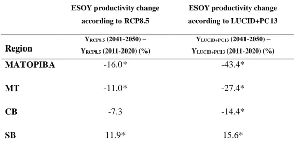
26 Our simulations also show that MATOPIBA is predicted to be the most affected region, and may lose 16% (43.4%) of ESOY productivity according to RCP8.5 (LUCID+PC13). MT and CB ESOY productivity are also negatively affected by climate change until 2050, and RCP8.5 simulations show a more moderate decrease (11 and 7.3%, respectively) than LUCID+PC13 (27.4 and 14.4%, respectively) (Table 1.3). As LUCID+PC13 land-use scenarios are more drastic than those of RCP8.5 in central-northern Brazil (MT, CB and MATOPIBA), this difference in productivity decrease between the two groups of simulations is probably related to a stronger negative biogeophysical signal associated to tropical deforestation.
In Southern Brazil, where the amount of deforested area is similar in RCP8.5 and LUCID+PC13, both groups of simulations agree that ESOY productivity may increase by 11.9-15.6% until the middle of the century (Table 1.3). In these cases, the change in precipitation from 2011-2020 to 2041-2050 is small (Figures 1.6-d), and this increase is most likely due to higher levels of CO2.
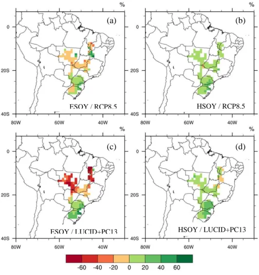
27 Figure 1.5– Percentage change in soybean yield from 2011-2020 to 2041-2050 after climate change. In (a) and (b) atmospheric composition and land use
trajectories are according CMIP5’s RCP8.5 scenario. In (c) and (d), atmospheric composition trajectories are according to CMIP5’s RCP8.5
scenario, but land use trajectories are according to Pires and Costa (2013) tropical deforestation scenarios.
(c) (d)
(a) (b)
ESOY / RCP8.5 HSOY / RCP8.5
28 In MATOPIBA, MT and CB, HSOY productivity may increase from 2.2 to 14.3% to according to RCP8.5. The increased productivity of these regions is limited to 2.3 to 6.2% according to LUCID+PC13 (Table 1.4). In general, southern states are the most favored (from 12.2 to 16.4% increase). We should note here that these increases in yield are most likely a consequence of the increased atmospheric CO2 concentration.
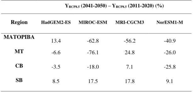
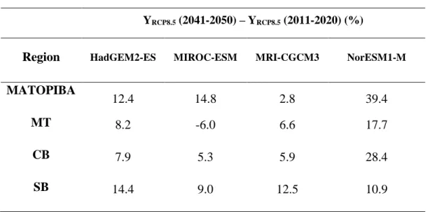
Table 1.3 – Change in soybean productivity from 2011-2020 to 2041-2050 for different Brazilian productive regions, for short cultivars (1600 GDD) planted in Sep 25th (ESOY). In the second column, both atmospheric composition and land-use change trajectories are according to RCP8.5. In the third column, atmospheric composition is according to RCP8.5 and land use change is according to (Pires and Costa, 2013).
ESOY productivity change
according to RCP8.5
ESOY productivity change
according to LUCID+PC13
Region
YRCP8.5 (2041-2050) –
YRCP8.5 (2011-2020) (%)
YLUCID+PC13 (2041-2050) –
YLUCID+PC13 (2011-2020) (%)
MATOPIBA -16.0* -43.4*
MT -11.0* -27.4*
CB -7.3 -14.4*
SB 11.9* 15.6*
29 Table 1.4 – Change in soybean productivity from 2011-2020 to 2041-2050 for different Brazilian productive regions, for optimum cultivar and planting date (HSOY). In the second column, both atmospheric composition and land-use change trajectories are according to RCP8.5. In the third column, atmospheric composition is according to RCP8.5 and land use change is according to (Pires and Costa, 2013).
HSOY productivity change
according to RCP8.5
HSOY productivity change
according to LUCID+PC13
Region
YMAX
RCP8.5 (2041-2050) –
YMAX
RCP8.5 (2011-2020) (%)
YMAX
LUCID+PC13 (2041-2050) –
YMAX
LUCID+PC13 (2011-2020) (%)
MATOPIBA 14.3* 2.3
MT 2.2* 2.8
CB 6.6* 6.2*
SB 12.2* 16.4*
30 Figure 1.6 – Change in precipitation (%) from 2011-2020 to 2041-2050 for the months of September, October, November and December for the different soybean productive regions considered in this study, as in RCP8.5 (circles and solid lines are the average and the models range, respectively) and LUCID+PC13 5 (triangles and dashed lines are the average and the models range, respectively). -70 -50 -30 -10 10 30 50 70
S O N D
(a) MATOPIBA -70 -50 -30 -10 10 30 50 70
S O N D
(b) MT -70 -50 -30 -10 10 30 50 70
S O N D
(c) CB -50 -30 -10 10 30 50
S O N D
(d) SB
RCP8.5 LUCID+PC13
31 1.3.2 Implications for double-cropping systems in central-northern Brazil
Our simulations strongly indicate that future climatic conditions may be unfavorable to early-planted soybeans in central-northern Brazilian productive regions, where ESOY productivity may decrease expressively until the middle of the century, regardless of the scenario. On the other hand, although climatic conditions become worse during the first dates of the crop calendar, Y improves for later dates (HSOY), showing that adapting planting dates can offset soybean productivity losses caused by climate change.
Based on the hypothesis that delaying planting dates improves productivity responses after climate change, we assess the opportunity to maintain highly productive double-cropping systems by delaying the soybean planting dates to times of the year when the climate may be more favorable. Although relatively simple, this may not be a straightforward analysis since, as mentioned before, commodity agriculture in central-northern Brazil happens in large ranches, where soybean cropland may be as extensive as 10,000 ha in a single ranch, and the sowing operation may last from 2 to 4 weeks to be completed. To simplify this analysis, we consider an average planting operation duration of ~3 weeks (20 days).
32 in these regions, which may negatively affect its productivity) we consider that there is a high probability that a double cropping system is viable when soybean, the first crop, reaches physiological maturity (when it can be harvested) by the beginning of January. Similarly, we consider that there is medium probability that a double-cropping system is still viable after climate change if soybean reaches physiological maturity by the middle of January, and after that date, double-cropping systems may become not be viable.
33 In MATOPIBA (Figure 1.7-a), according to RCP8.5 delaying the beginning of the planting operation to October 5 in 2041-2050 may lead to an increase of Y (relative to soybean planted in 09/25 in the first decade - Y09/25(2011-2020)) during virtually all the planting operation. But, in this case, there is medium to low probability that a double-cropping system is viable in this region by the middle of the century. However, according to LUCID+PC13 delaying the beginning of the planting operation to October 5 in 2041-2050 may lead to a decrease of Y in the first 10 days of the planting operation (as opposite to RCP8.5) and to a moderate increase in Y for the last 10 days. In this case, a double-cropping system would be viable only in half of the large farms (those planted until October 15). Delaying the beginning of the planting operation to later than October 15 still does not allow a second crop, but soybean productivity is higher due to favorable climatic conditions and increased atmosphere CO2 concentration.
34 Figure 1.7 – Soybean productivity change [Yd(2041-2050) / Y09/25(2011-2020), where d
are the planting dates assessed in this study] after climate change. Full black boxes (circles) represent soybean planting dates that lead to a high probability of double-cropping viability according to RCP8.5 (LUCID+PC13). Full gray boxes (circles) represent soybean planting dates that lead to a medium probability of double-cropping viability, also according to RCP8.5 (LUCID+PC13). Empty boxes (circles) represent soybean planting dates that may lead to unviable double-cropping according to RCP8.5 (LUCID+PC13). Dashed boxes indicate the sowing windows.
1/4 1/2 1 2 4 (b) MT 1/4 1/2 1 2 4 (a) MATOPIBA
□
RCP8.5○ LUCID+PC13
35 1.4 CONCLUSIONS
Sowing early soybean cultivars right after the end of the sanitary break has been economically attractive for Brazilian farmers in recent years: the probability of infection with rust is low, early cultivars remain less time in the field and less time exposed to infection, the market prices for soybean harvested earlier is higher than in the peak of harvesting season, and there is the climatic possibility to plant a second crop in the same agricultural calendar. Usually, profit offsets the risk of sowing soybean under uncertain climatic conditions (mainly precipitation) in the beginning of the rainy season.
However, the results of this assessment strongly suggest that the average climate risk may increase for soybean planted right after the end of the sanitary break in the main productive regions in Central/Northern Brazil until 2050, regardless of the scenario or climate model used. This result is associated to an important reduction of precipitation during the transition months from the dry to the wet season, when double-cropping farmers are sowing soybean. As expected, the positive physiological effects of increased atmospheric CO2 concentration is not sufficient to offset the negative effects of dry conditions during the early soybean cycle. In addition, more severe deforestation levels may lead to sharper decreases in productivity until 2050, indicating that the expansion of the agricultural frontier may cause negative feedbacks on agricultural productivity.
36 technique, but it decreases the probability to plant a second crop in the same land in the same agricultural calendar. Again, stronger deforestation levels limits productivity responses and may lead to more moderate increase in productivity than in lower deforestation levels.
In case farmers still choose to adopt viable double-cropping systems in central Northern Brazil, the future sowing windows would have to narrow substantially (to 10 days, at maximum) in the case of large farms that currently need several weeks to complete the planting operation. Therefore, the simulations in this study indicate that the sustainability of double-cropping systems may be threatened in central Northern Brazil, and that clearing additional to area to offset productivity loss may cause negative feedbacks on the existing farms, further decreasing soybean productivity.
In contrast, sowing soybean in November-December, when rainfall conditions are more favorable, may reduce climate risk and even expressively increase productivity in Southern Productive regions since soybean photosynthetic processes may be favored in a high atmospheric CO2 scenario. Nevertheless, sowing later in November-December may also imply in an increased phytosanitary risk when compared to the early sowers, and on unviable double-cropping systems, and the total grain output (soybean + maize) would significantly decrease in these regions.
37 without adaptation, the total soybean + maize output may not be sustainable in some productive regions in Brazil until the middle of the century.
In the view of this scenario, effective adaptation strategies are required. Some suggestions of adaptation strategies to maintain highly productive double-cropping systems until the middle of the century are:
technological solutions focused on the initial stages of soybean cycle, especially for early cultivars, when water deficit will be larger (for example, new drought tolerant seeds to current cultivars, or the development of new drought tolerant cultivars);
investment in productive early soybean and maize cultivars (90-100 days cycle each) – such cultivars do exist today, but have low yields;
and the incorporation of climate prediction in the Climate Risk Agricultural Zoning (or Zoneamento Agrícola De Risco Climático, in portuguese) recommendations. These recommendations, that are criteria for agricultural credit in Brazil, are based on past climate time-series and may miss some the dynamics introduced by climate change, especially the shortening of the rainy season.
38 on the yields. In other words, large-scale agriculture expansion in northern Brazil leads to the degradation of the climate regulation ecosystem it relies on.
39 CHAPTER 2
EFFECTS OF CLIMATE CHANGE IN PASTURE PRODUCTIVITY AND IMPLICATIONS FOR LAND USE IN BRAZIL
2.1 INTRODUCTION
The past development of agriculture in Brazil has been intimately connected with the substitution of natural biomes by pasturelands. The main reason why cattle ranching was the most usual activity driving the extension of agricultural frontiers in Brazil is that it is the least expensive and most efficient way to occupy and ensure ownership of large expansions of land (Bowman et al., 2012; Dias-Filho, 2013; Lapola et al., 2014). Due to the intensive grazing and low levels of technology adoption, these pasturelands would quickly become unproductive and were usually left behind or occupied by new agricultural uses. This process persisted for many years and resulted in a large herd that is fed essentially with pastures in low-productive cattle ranches, which contrasts with the high yields observed in many crops in the country.
40 As the current pasturelands are underproductive (in terms of heads per hectare), a great opportunity to sustainably increase productivity is to close yield gaps on the existing farms while breaking the cycle of environmental degradation (Foley et al., 2011). Such farms could expressively increase productivity with the combination of the adoption of relatively simple management practices such as cattle rotation and pasture fertilization, as recommended by EMBRAPA (Empresa Brasileira de Pesquisa Agropecuária) and economic policies, as a tax on cattle from conventional pasture and a subsidy for cattle from semi-intensive pasture (Cohn et al., 2014). In these cases, productivity on the existing farms could increase by 2.5-fold in comparison to conventional systems and spare land for deforestation. Such elements have been extensively studied and applied in experimental farms in Brazil, but have not yet been widely adopted.
41 Here we conduct an updated assessment of the effects of climate change until 2050 in pasture productivity in the main productive regions in Brazil. We use a calibrated large-scale ecosystem model to assess the effects of a high emission scenario (RCP8.5), and contrast it to an alternative scenario where levels of deforestation in Amazonia and Cerrado are increased. The results presented here may be critical to assess the sustainability of forage availability on the existing farms in Brazil and if the previously proposed solutions (management and economic incentives) to increase meat production in Brazil may be effective, even in a future climate change scenario.
2.2 MATERIALS AND METHODS
2.2.1 Productive regions
We evaluated individually the results of pasture productivity change in the main cattle productive regions in Brazil (Figure 2.1), identified by the following acronyms: Northern Brazil (NB); aggregating results from Mato Grosso, Pará and Rondônia states; MATOPIBA, which aggregates results for Maranhão, Tocantins, Piauí and Bahia states; Central Brazil (CB), with results from Mato Grosso do Sul, Goiás, Minas Gerais and São Paulo states; and Southern Brazil (SB), for Paraná, Santa Catarina and Rio Grande do Sul. Together, these regions hold about 90% of the total Brazilian herd in 2014 (Table 2.1).
42 Figure 2.1 – Analyzed productive regions. Each 1o x 1o pixel shown here had at least 10%
of its area covered by pasturelands in 2012.
Table 2.1 – Main cattle productive regions in Brazil and their total production (IBGE, 2015). Total Brazilian production in 2014 is 2.12x10⁸ heads.
Region Acronym Production in 2014 (heads) Brazilian production % from total in 2012
Maranhão, Tocantins,
Piauí and Bahia MATOPIBA
2.8 x 10⁷ 13.33
Northern Brazil NB 6.1 x 10⁷ 28.84
Central Brazil CB 7.6 x 10⁷ 35.97
Southern Brazil SB 2.7 x 10⁷ 12.92
43 2.2.2 Climate models and input data
Essentially, the simulated climates of the same four Earth System Models from CMIP5 used to simulate soybean productivity (section 1.2.2) were used to estimate future pasture productivity – HadGEM2-ES, MIROC-ESM, MRI-CGCM3 and NorESM1-M (Table 1.1). Reassessment of the annual precipitation cycle for the pasture planted area in Brazil indicates that these models simulate, in average, monthly precipitation according to GPCP from January to June. However, from July to December, ESMs generally underestimate precipitation in pasture areas in Brazil (Figure 2.1).
44 Figure 2.2 – Daily mean precipitation for each month of the period 1979-2000 as in GPCP and as simulated by the models: MIROC-ESM, MRI-CGCM3, NorESM1-M and HadGEM2-ES. The monthly averages are calculated over each one of the soybean productive regions in Brazil.
2.2.3 Pasture model description
The simulations of pasture productivity were run with the same surface model used for the estimation of soybean productivity (Chapter 1), the Integrated Model of Land Surface Processes (INLAND). As mentioned before, the version used in this study
0 2 4 6 8 10 12 14 Ja n Feb Ma r A pr Ma y
Jun Jul Aug Sep Oct Nov Dec (d) SB NorESM1-M HadGEM2-ES MRI-CGCM3 MIROC-ESM 0 2 4 6 8 10 12 14 Ja n Feb Ma r A pr Ma y
Jun Jul Aug Sep Oct Nov Dec (c) CB GPCP Ensemble 0 2 4 6 8 10 12 14 Ja n Feb Ma r A pr Ma y
Jun Jul Aug Sep Oct Nov Dec b) NB 0 2 4 6 8 10 12 14 Ja n Feb Ma r A pr Ma y
45 (version 2.0) includes the representation of 16 plant functional types (PFTs): 12 of them are natural (one of which was used to simulate the growth of pastureland as C4 grasses), and the remaining four are crops (soybeans, corn, wheat and sugarcane).
Crops and natural ecosystems share the same Equations to simulate the balance of energy and mass, which operates at scales ranging from 60 minutes to 1 year (Foley et al., 1996). However, the methodology for the simulation of phenology and carbon allocation are different for natural and agricultural ecosystems. For natural ecosystems plant functional types, net primary production (NPP) is calculated through the integration of primary production throughout the year and discounting maintenance and growth respiration. Then, NPP is allocated in three carbon pools: leaves (CL), wood and roots. The changes in the leaf carbon pool are expressed by the differential Equation 2.1 (Senna, 2008):
���
�� = ����� −
��
�� − �. �� (2.1)
46 The model was calibrated using data from a field experiment held in Viçosa (20º 45' S; 42º 52' W), where Brachiaria brizantha cv. Marandu was cultivated from September 2013 to April 2014 in no-grazing conditions. Prior to sowing, soil was prepared conventionally, fertilized and had acidity controlled. Using the data from that experiment, the model was optimized to CL. The leaf area index (LAI) of each PFT is obtained by dividing leaves carbon (CL) by specific leaf area. In this study, we derived the specific leaf area parameter from field data experiment, which was set to 6 m2.kgC-1. The calibration process involved executing a large number of simulations and, in each one of them, a different value for ��. In each simulation, the results of the simulated CL are compared against observed filed data, seeking to minimize the mean absolute error (MAE). The optimum value of ��and used in INLAND simulations was 2.4 years.
The simulations with the calibrated model of pasture productivity were also run for the entire South America, with a grid resolution of 1ox1o (~110km x 110km).
2.2.4 Experiment design
2.2.4.1Land use and climate change scenarios
47 2.2.4.2 Significance tests
For each group of simulations described in section 1.2.4.2, we averaged the outputs of simulations of all ensembles and created an average time-series (from 2011 to 2050) of pasture productivity (P, kgC.ha-1yr-1), therefore reducing the uncertainty and model-related bias. We then calculated the percentage change (Equation 2.2) and tested the hypothesis that the average pasture productivity changes from the first to the last decade in the 2011-2050 period due to climate change.
∆� % = ( � −� − � −
− ) � (2.2)
In other words, we test the hypothesis that pasture productivity in 2041-2050 (P2041-2050) is different from the average soybean productivity in 2011-2020 (P2011-2020), being that difference related to the climate change that occurred between these periods.
We used the Student’s t test, with a 5% level of significance and n = 10 years to test this
hypothesis, in the two groups of simulations described in section 1.2.4.2.
2.3 RESULTS
48 productivity for each individual climate model used is available in Appendix A (Figures A5, A6, A7 and A8 and Tables A5 and A6).
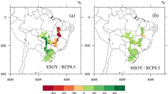
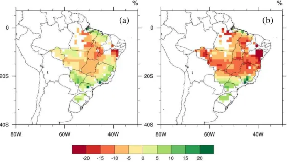
In RCP8.5, pasture productivity decreases modestly in most of the study area, ranging from 0 to 10% decrease, except for southern Bahia and northern Minas Gerais, where the reductions are slightly higher and reach values close to 15% (Figure 2.3-a). However, although for LUCID+PC13 simulations, where deforestation levels are higher, the general spatial patterns of pasture productivity decrease resembles the results from RCP8.5 simulations, it declines more sharply. The most affected regions are located in an area extended from southern to northern cost of Bahia state, northeastern Minas Gerais, western Mato Grosso, Mato Grosso do Sul and Rondônia states, where it decreases more than 20% from 2011-2020 to 2041-2050 (Figure 2.3-b).
In addition, in southern regions pasture productivity slightly increases (< 5 %) according to both RCP8.5 and LUCID+PC13 simulations.
49 Figure 2.3 – Percentage change in pasture productivity from 2011-2020 to 2041-2050 after climate change. In (a) atmospheric composition and land use trajectories are
according CMIP5’s RCP8.5 scenario. In (b) atmospheric composition trajectories are according to CMIP5’s RCP8.5 scenario, but land use trajectories are according to Pires and Costa (2013) tropical deforestation scenarios.
In contrast to the other regions, SB pasture productivity is predicted to slightly increase until 2050 according to simulations. This simulated slight increase, although not statistically significant, may be a consequence of the increased CO2 atmospheric concentration (Table 2.2).
50 Table 2.2 – Change in pasture productivity from 2011-2020 to 2041-2050 for different Brazilian productive regions. In the second column, both atmospheric composition and land-use change trajectories are according to RCP8.5. In the third column, atmospheric composition is according to RCP8.5 and land use change is according to (Pires and Costa, 2013).
Pasture productivity change
according to RCP8.5
Pasture productivity change
according to LUCID+PC13
Region PRCP8.5 (2041-2050) – PRCP8.5 (2011-2020) (%)
PLUCID+PC13 (2041-2050) –
PLUCID+PC13 (2011-2020) (%)
MATOPIBA -6.0* -11.5*
NB -4.0* -10.4*
CB -3.4 -9.2*
SB 2.1 3.4
(*) Statistically significant according to Student’s t test, α=5% (n = 10).
51 Figure 2.4 – Change in yearly precipitation (mm/yr) from 2011-2020 to 2041-2050 after climate change to the most productive Brazilian regions, as in RCP8.5 (circles and solid lines are the average and the models range, respectively) and LUCID+PC13 5 (triangles and dashed lines are the average and the models range, respectively).
2.4 DISCUSSION AND CONCLUSIONS
Clearing and burning natural forests and savannas and replacing it by cattle ranches has been the main driver of agricultural expansion and environmental degradation in central-northern Brazil. As a low-cost manner to own land, the implementation of pastures were the main primary use of land after deforestation, and were pushed into new areas whereas gradually replaced by other agricultural uses, as soybeans, for example. As
-400 -300 -200 -100 0 100 200
MATOPIBA NB CB SB
Pre ci pi tat io n cha ng e f rom 2011 -2020 to 2041 -2050 (m m /y r)
52 a result, it currently represents around 68% of the total agricultural area in Brazil, with a great share of degraded and underproductive pasturelands due to the long-lasted unsustainable use of land resources.
Given this current scenario, it is clear that to increase total meat output while meeting sustainability needs requires the restoration of vast areas of degraded pasture and improvements in cattle management practices. Such practices have been shown to be successful when tested in Brazilian experimental farms, but not extensively adopted by farmers. However, besides management practices there is another factor that may determine the successful increase in cattle meat output in the future: climate change.
53 Zimmer (2011) show that the recovery of degraded pastures in Mato Grosso can increase stocking rate by 2.6 times.
Despite the limited negative impact in pasture productivity in the most productive Brazilian regions, this study demonstrates that the increased productivity loss for higher deforestation levels reinforces the recommendations of intensification of cattle ranching in the existing low-productive farms – a country average 1.36 heads per hectare in 2010 (IBGE, 2010) – as a win-win strategy. Intensification, as opposed to extensification, brings obvious ecological benefits (less environmental degradation and biodiversity preservation, for example) but also directly benefits crops through climate regulation, an ecosystem service that agriculture relies on.
Finally, these results reinforce the need to continue and to expand important governmental public policies and programs that directly or indirectly help to curb the expansion of the agricultural frontier in central-northern Brazil and to preserve the services it provides. Examples of existing programs that aim to directly curb deforestation are: (i) the Action Plan for Prevention and Control of Deforestation in the Legal Amazon (Plano de Ação para Prevenção e Controle do Desmatamento na Amazônia Legal – PPCDAm); (ii) the Action Plan for Prevention and Control of Deforestation and Fires in the Cerrado (Plano de Ação para Prevenção e Controle do Desmatamento e das
Queimadas no Cerrado - PPCerrado). In addition, as important to sustainable livestock
55 CHAPTER 3
GENERAL CONCLUSIONS
3.1 THESIS OVERVIEW
The world will face the challenge to feed more than 2 billion additional people until the middle of this century while agriculture moves to a new standard of not driving environmental degradation and while severe climate changes take place, and Brazilian agriculture will play an important role to achieve this goal. Currently, greenhouse gas
emissions are high and very close to IPCC’s most pessimistic scenario (Fuss et al., 2014)
and there is limited evidence that deforestation in Brazil is coming to its end (Lapola, et
al., 2014).
This thesis investigates if the effects of these two forcings ‒ global climate change until the middle of the century and additional deforestation ‒ will affect the productivity of the main agricultural commodities produced in Brazil (soybeans and cattle pasture) using the climate simulated by four climate models in two different climate change scenarios as input to a gridded crop model. To study this subject, this thesis is divided in two chapters, one for each crop, and the conclusion of each chapter is summarized below.